Optimising DAX: Model Design Comparisons and Testing Tips


Hello again. Over the last few posts in the Optimising DAX series, we've covered how VertiPaq stores data, encoding techniques, cardinality, and relationship costs. In this post, we're putting it all together to compare three common model designs and see how they perform in practice.
The Comparison
During the workshop, we loaded the same data into three different model designs in DAX Studio and compared the results:
Star Schema - Dimension tables (customers, products, dates) linked to a central fact table. Flat Table - Everything denormalised into a single wide table. Header/Detail - Two fact tables linked by a primary key.
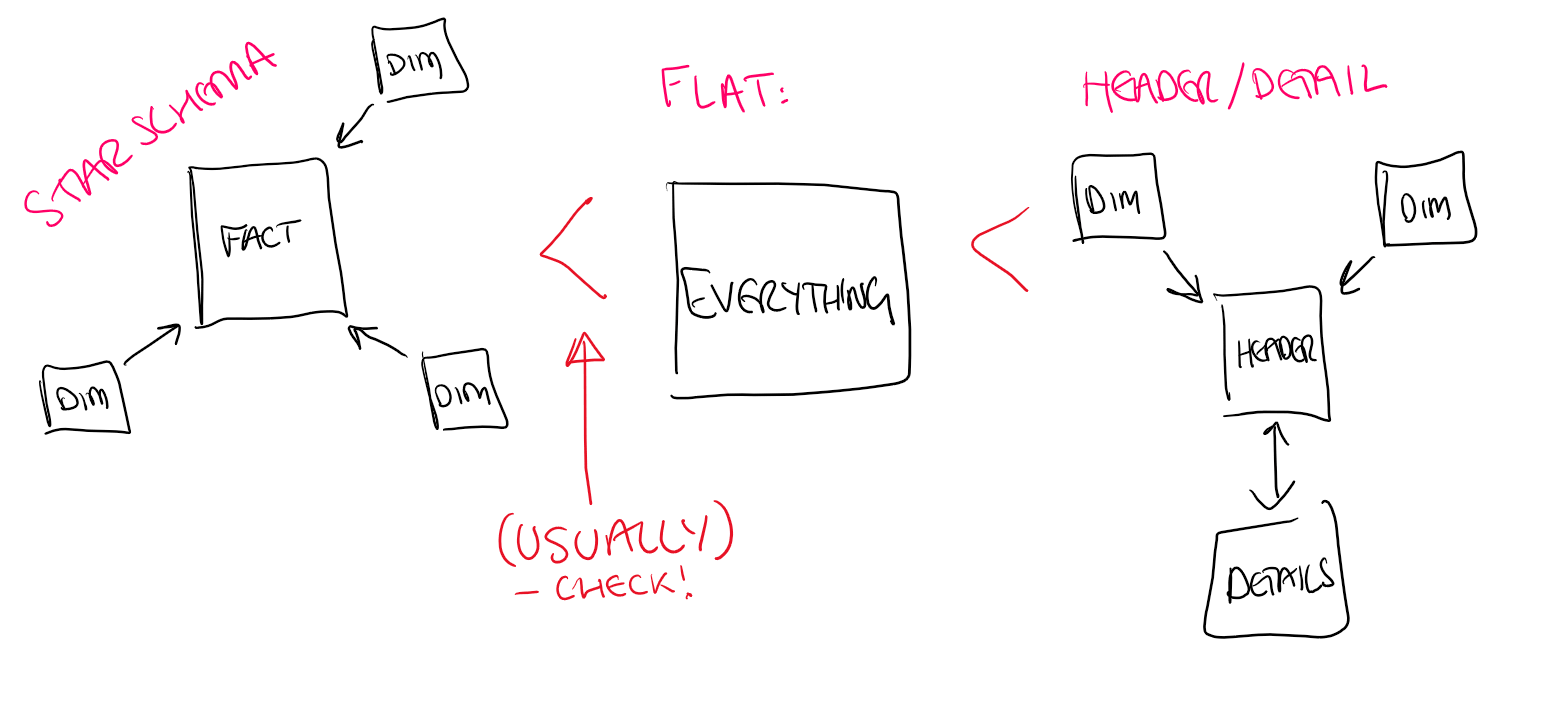
In the example, star schema was the smallest, then flat table, then header/detail. Though it's always worth checking with your specific data!
Why Star Schema Wins
The dimension tables are small and compress well. The fact table contains foreign keys (medium cardinality) and measures. Everything benefits from good compression, and the relationships are through relatively low-cardinality keys.
Why Flat Tables Are Actually Okay
In a flat table, a lot more values are repeated. This sounds wasteful, but all those repeated customer names and product categories actually compress quite well via run-length encoding (if the sort order works out). The main downsides are that there are more columns to analyse for sort order (remember the 10-second budget), and scans over the flat table are bigger than scans over small dimension tables.

Why Header/Detail Is Usually Worst
The link between the two tables is an ID column - so with 100% cardinality, the biggest column is then repeated twice in the model. It gets almost no compression benefit. On top of that, every query traverses this high-cardinality relationship. As we discussed in the previous post: linking two large fact tables via their primary key is about the worst thing you can do.
Calculated Columns: Sometimes Helpful
Calculated columns have a bit of a bad reputation, and sometimes fairly. They increase model size and are computed during refresh. But there are cases where they can improve query performance.
Calculated columns can sometimes be a good idea, especially if the calculated column has lower cardinality than the columns it's derived from. For example, bucketing a high-precision decimal into ranges ("0-10", "10-20", etc.) creates a much lower-cardinality column that's faster to scan and filter.
But there really aren't any set rules here. Whether it helps depends on your data and queries - it always requires trying and testing.

Testing Tips
A few practical things from the workshop:
Use real data for model testing. The distribution of values matters hugely for compression, so synthetic or sampled data can give misleading results.
Enable Server Timings in DAX Studio to see how long different operations take. Scanning different columns takes different amounts of time - if you do a SUM over a column with high cardinality, it will take noticeably longer. A direct consequence of the compression mechanics.
Measure, don't guess. Your intuition about which columns are problematic isn't always right. DAX Studio shows you what's actually happening.
What's Next
That wraps up the model optimisation half of the series. Look out for the next post on how the formula engine and storage engine work together when you actually execute a DAX query.