Polars Workloads on Microsoft Fabric
TL;DR: Run fast, cost-effective analytics on Microsoft Fabric without Spark clusters by using Polars. This guide covers reading from OneLake, transforming data with lazy evaluation, writing to Delta tables, and seamlessly switching between local and Fabric environments.
Overview
Microsoft Fabric's Python Notebooks provide an ideal environment for running Polars-based analytics workloads. With Polars pre-installed and native access to OneLake, you can build fast, memory-efficient data pipelines without the overhead of Spark. This post walks through the practicalities: reading raw files, transforming data, and writing to Delta tables in your Lakehouse.
Key points:
- Reading files: Use relative paths (
/lakehouse/default/Files/...) for the pinned lakehouse, or ABFS paths for cross-workspace access - Reading Delta:
pl.read_delta()orpl.scan_delta()for lazy evaluation - Writing Delta:
df.write_delta()works out of the box; usedt.replace_time_zone("UTC")on timestamps to avoid SQL endpoint errors - Storage options: Only needed for cross-lakehouse access—pass
{"bearer_token": notebookutils.credentials.getToken('storage'), "use_fabric_endpoint": "true"} - Performance: Use
scan_*methods for large files, specify columns upfront, and consider tuning rowgroups (8M+ rows) for DirectLake consumption - Limitations: No V-ORDER or Liquid Clustering without Spark; max 64 vCores on single node
Why Polars on Fabric?
Fabric's new Python Notebooks run on a lightweight single-node container (2 vCores, 16GB RAM by default) rather than a Spark cluster. This is a better fit for many workloads:
- Speed without complexity: Polars' Rust-based engine delivers Spark-comparable performance on datasets that fit in memory, without the cluster coordination overhead.
- Cost efficiency: No Spark cluster spin-up means lower CU consumption for smaller jobs.
- Rapid iteration: Sub-second notebook startup times versus minutes for Spark.
- Seamless integration: Polars is pre-installed and OneLake paths work out of the box.
Microsoft explicitly recommends Polars (alongside DuckDB) as an alternative to pandas when you encounter memory pressure—a tacit acknowledgement that single-node, in-process tools have earned their place in the enterprise data stack.
Writing code that can run both locally and on Fabric
One of the major benefits that we find in using Polars is that we can develop locally (using local compute and local storage) and then deploy onto Fabric for fully hosted, production scale, automated operations.
This gives us the best of both worlds: a developer experience that feels like mainstream software engineering (fast inner dev loop with local unit tests which run in seconds), and the ability to deploy onto a cloud platform for orchestration and integration into the wider enterprise data pipeline ecosystem.
But in order to do this, we need to set up a simple helper function to detect where the code is running and set up the connections accordingly.
We tackle this in a few stages.
Firstly we need to detect if the code is running in a Fabric Python Notebook, we can determine that by checking for specific environment variables as follows:
import os

def is_fabric_python_notebook() -> bool:
    """Detect specifically a Python (non-Spark) notebook."""
    return (
        'JUPYTER_SERVER_HOME' in os.environ
        and 'SPARK_HOME' not in os.environ
    )

logger.info(f"Is this running in a Fabric Python Notebook?: {is_fabric_python_notebook()}")
INFO: Is this running in a Fabric Python Notebook?: False
Next we need to be able to construct an abfss (Azure Blob File System Secure) path to files / folders that we want to be able to read from or write to using Polars.
The format of an abfss path adopts the following convention on Fabric:
abfss://{ws}@onelake.dfs.fabric.microsoft.com/{lh}.Lakehouse
Where {ws} is replaced by the Fabric workspace name and {lh} is replaced by the lakehouse name.
Furthermore, Fabric lakehouses are organised into two discrete areas:
- Files - an area which is used to hold raw or unstructured content. It has an
abfsspath:abfss://{ws}@onelake.dfs.fabric.microsoft.com/{lh}.Lakehouse/Files/{relative_path} - Tables - an arae which holds tabular data (most commonly in Delta format). It uses an
abfsspath convention of:abfss://{ws}@onelake.dfs.fabric.microsoft.com/{lh}.Lakehouse/Tables/{schema_name}/{table_name}
There is also an option to "pin" a default lakehouse to a Fabric notebook and reference that in a shorthand path as follows:
- Files:
/lakehouse/default/Files/{relative_path} - Tables:
/lakehouse/default/Tables/{schema_name}/{table_name}
It can be convenient to use this pinned default lakehouse for exploratory data analysis in notebooks. However for software that is destined to end up in production, we recommend using the full abfss path to explicitly reference the lakehouse.
Furthermore, you can only pin one lakehouse to a notebook, this doesn't work well with the common pattern we see where a notebook is reading from one lakehouse (e.g. "Bronze"), wrangling the data and writing out to another lakehouse (e.g. "Silver"). For this reason, it makes sense to declare the full abfss path for both the sync and target lakehouses just to keep things consistent.
So it is often useful to use a Python helper function to construct the abfss path from component parts:
def construct_base_abfss_path(workspace_name: str, lakehouse_name: str) -> str:
    """Construct the base ABFSS path for a given workspace and lakehouse."""
    # Because it is a URL, replace spaces with %20
    workspace_name = workspace_name.replace(" ", "%20")
    lakehouse_name = lakehouse_name.replace(" ", "%20")
    return f"abfss://{workspace_name}@onelake.dfs.fabric.microsoft.com/{lakehouse_name}.Lakehouse"
construct_base_abfss_path(workspace_name="polars_demo_workspace", lakehouse_name="polars_demo_lakehouse")
'abfss://polars_demo_workspace@onelake.dfs.fabric.microsoft.com/polars_demo_lakehouse.Lakehouse'
Finally, we need to pass the "storage options" information to Polars to enable it to read from or write to a Fabric lakehouse.
The storage_options parameter is a dictionary which needs to contain two named elements:
- bearer_token - that will enable Polars to authenticate with the Fabric lakehouse API
- use_fabric_endpoint - set to value "true" to tell Polars to leverage the fabric endpoint
The notebookutils Python package is installed in the Python environment used by Fabric notebooks. This enables you to retrieve the bearer token.
import notebookutils
storage_options = {
    "bearer_token": notebookutils.credentials.getToken('storage'),
    "use_fabric_endpoint": "true"
}

df.scan_csv(
    f"abfss://polars_demo_workspace@onelake.dfs.fabric.microsoft.com/polars_demo_lakehouse.Lakehouse/Files/land_registry_data/*.csv",
    storage_options=storage_options
)
Putting this all together, we can now set up the paths we will read from and write to using Polars dynamically based on whether we are running the notebook locally or on Fabric:
- Detect if we are running the notebook in Fabric (specifcally testing to see if it is a Python notebook)
- Build the base path:
- An
abfsspath if we are running on Fabric - A standard file path if we are running locally
- An
- Additionally, if running on Fabric, import and leverage the
notebookutilspackage to authenticate and generate a token that will enable connection to the lakehouses (provided we have permissions to do so) - Construct paths as required for source(s) and target(s) - in this case, we are keeping things simple:
- We are reading from and writing to the same workspace / lakehouse
- We are reading from one source (a folder containing *.csv files)
- We are writing to a three target tables: house_prices, dates and locations
class FabricPaths:

    def __init__(self, workspace_name: str, lakehouse_name: str, local_base_path: str = "data/fabric"):
        self.workspace_name = workspace_name
        self.lakehouse_name = lakehouse_name
        self.local_base_path = local_base_path
        self.is_fabric = FabricPaths._is_fabric_python_notebook()

        if self.is_fabric:
            import notebookutils  # This Python package is only available on Fabric, so we need to import it conditionally.

    def generate_file_path(self, relative_path: str) -> str:
        """Generate a full file path for the given folder type and name."""
        base_path = self._construct_base_abfss_path()
        return f"{self._get_base_path()}/Files/{relative_path}"

    def generate_table_path(self, schema_name: str, table_name: str) -> str:
        """Generate a full table path for the given schema and table name."""
        base_path = self._construct_base_abfss_path()
        return f"{self._get_base_path()}/Tables/{schema_name}/{table_name}"

    def get_storage_options(self):
        """Get storage options for accessing Fabric storage."""
        if self.is_fabric:
            storage_options = {
                "bearer_token": notebookutils.credentials.getToken('storage'),
                "use_fabric_endpoint": "true"
            }
        else:
            storage_options = {}
        return storage_options

    def _get_base_path(self) -> str:
        """Get the appropriate base path depending on the environment."""
        if self.is_fabric:
            return self._construct_base_abfss_path()
        else:
            return self.local_base_path

    @staticmethod
    def _is_fabric_python_notebook() -> bool:
        """Detect specifically a Python (non-Spark) notebook."""
        return (
            'JUPYTER_SERVER_HOME' in os.environ
            and 'SPARK_HOME' not in os.environ
        )

    def _construct_base_abfss_path(self) -> str:
        """Construct the base ABFSS path for a given workspace and lakehouse."""
        # Because it is a URL, replace spaces with %20
        workspace_name = self.workspace_name.replace(" ", "%20")
        lakehouse_name = self.lakehouse_name.replace(" ", "%20")
        return f"abfss://{workspace_name}@onelake.dfs.fabric.microsoft.com/{lakehouse_name}.Lakehouse"
# Now use this class to generate paths

# We only need one class because we are working within a single Fabric workspace and lakehouse
fabric_paths = FabricPaths(
    workspace_name="polars_demo_workspace",
    lakehouse_name="polars_demo_lakehouse",
    local_base_path="../data/fabric"
    )

# Generate paths
raw_data_download_path = fabric_paths.generate_file_path("land_registry_data")
logger.info(f"Path to download CSV files into: {raw_data_download_path}")

source_path = fabric_paths.generate_file_path("land_registry_data/*.csv")
logger.info(f"Glob path to read all CSV files: {source_path}")

target_path_prices = fabric_paths.generate_table_path("house_price_analytics", "prices")
logger.info(f"Target table path for price fact table: {target_path_prices}")

target_path_dates = fabric_paths.generate_table_path("house_price_analytics", "dates")
logger.info(f"Target table path for date dimension table: {target_path_dates}")

target_path_locations = fabric_paths.generate_table_path("house_price_analytics", "locations")
logger.info(f"Target table path for location dimension table: {target_path_locations}")

storage_options = fabric_paths.get_storage_options()
logger.info(f"Storage options for accessing Fabric storage: {storage_options}")
When running locally, this generates the following log:
INFO: Path to download CSV files into: ../data/fabric/Files/land_registry_data
INFO: Glob path to read all CSV files: ../data/fabric/Files/land_registry_data/*.csv
INFO: Target table path for price fact table: ../data/fabric/Tables/house_price_analytics/prices
INFO: Target table path for date dimension table: ../data/fabric/Tables/house_price_analytics/dates
INFO: Target table path for location dimension table: ../data/fabric/Tables/house_price_analytics/locations
INFO: Storage options for accessing Fabric storage: {}
When running in a Fabric Python Notebook, it generates the following log:
Path to download CSV files into: abfss://polars_demo_workspace@onelake.dfs.fabric.microsoft.com/polars_demo_lakehouse.Lakehouse/Files/land_registry_data
Glob path to read all CSV files: abfss://polars_demo_workspace@onelake.dfs.fabric.microsoft.com/polars_demo_lakehouse.Lakehouse/Files/land_registry_data/*.csv
Target table path for price fact table: abfss://polars_demo_workspace@onelake.dfs.fabric.microsoft.com/polars_demo_lakehouse.Lakehouse/Tables/house_price_analytics/prices
Target table path for date dimension table: abfss://polars_demo_workspace@onelake.dfs.fabric.microsoft.com/polars_demo_lakehouse.Lakehouse/Tables/house_price_analytics/dates
Target table path for location dimension table: abfss://polars_demo_workspace@onelake.dfs.fabric.microsoft.com/polars_demo_lakehouse.Lakehouse/Tables/house_price_analytics/locations
Storage options for accessing Fabric storage: {'bearer_token': '[REDACTED]', 'use_fabric_endpoint': 'true'}
That's it! The rest of the code is identical for both environments: we use the helper class above to take care of the only things that need to change: how the path is formed and setting up the storage_options for connecting in OneLake.
This class can become more sophisticated, for example:
- Adding a third option: run code locally, but connect to Fabric lakehouse for reading and writing data
- Handling for default pinned lakehouses
- Checking the workspace and lakehouse specified exist by calling Fabric APIs
- Wrapping the logic above into a package and deploying it on Fabric so it is available across all notebooks
But we have kept it simple in this case to illustrate the key concepts.
Download data
To support this use case, we are going to download some open data prime the "files" area with raw data we can analyse.
The are sourcing this from the UK Land Registry House Price Data open data repository.
Data is available for us under an Open Government Licence.
import requests
import fsspec

HOUSE_PRICE_BASE_URL = "http://prod.publicdata.landregistry.gov.uk.s3-website-eu-west-1.amazonaws.com/"

# Each file is approximately 100MB in size.  Change the number of years to control the total data size.
NUMBER_OF_YEARS = 3

list_of_files = [f"pp-{year}.csv" for year in range(2025, 2025 - NUMBER_OF_YEARS, -1)]

for file_name in list_of_files:

    remote_file_url = f"{HOUSE_PRICE_BASE_URL}{file_name}"
    path_to_save_file = raw_data_download_path + "/" + file_name

    # Download the CSV file with streaming enabled to avoid OOM on limited memory
    with requests.get(remote_file_url, stream=True) as response:
        response.raise_for_status()  # Ensure we notice bad responses

        # fsspec automatically handles the protocol (file:// versus abfss://) based on the source_path
        with fsspec.open(path_to_save_file, mode='wb', **storage_options) as f:
            # Write in 1MB chunks
            for chunk in response.iter_content(chunk_size=1024*1024):
                f.write(chunk)

    logger.info(f"Downloaded {file_name} to: {path_to_save_file}")
INFO: Downloaded pp-2025.csv to: ../data/fabric/Files/land_registry_data/pp-2025.csv
INFO: Downloaded pp-2024.csv to: ../data/fabric/Files/land_registry_data/pp-2024.csv
INFO: Downloaded pp-2023.csv to: ../data/fabric/Files/land_registry_data/pp-2023.csv
Reading files
When you create a new Python Notebook in Fabric you get immediate access to:
- Polars (currently v1.6 in the default environment)
- The
delta-rslibrary for Delta Lake operations
You can use all of the common Polars functions to read files from a Fabric lakehouse both eager and lazy versions:
| Format | Eager Read | Lazy Read | Eager Write | Lazy Write |
|---|---|---|---|---|
| CSV | pl.read_csv() |
pl.scan_csv() |
df.write_csv() |
lf.sink_csv() |
| Excel | pl.read_excel() |
❌ | df.write_excel() |
❌ |
| Parquet | pl.read_parquet() |
pl.scan_parquet() |
df.write_parquet() |
lf.sink_parquet() |
| JSON | pl.read_json() |
❌ | df.write_json() |
❌ |
| NDJSON | pl.read_ndjson() |
pl.scan_ndjson() |
df.write_ndjson() |
lf.sink_ndjson() |
| Delta | pl.read_delta() |
pl.scan_delta() |
df.write_delta() |
💡 coming soon? |
The reason you don’t see a sink_delta() method in Polars for Python is that it’s very new and not yet part of the stable public API. It was introduced in late 2025 in Polars’ Rust core to allow streaming writes directly to Delta Lake without collecting all data in memory first.
As of the last stable release (early 2026), the Polars Python package does not expose LazyFrame.sink_delta() or DataFrame.sink_delta() in the public API. The Polars team has indicated that sink_delta will likely appear in future stable releases once the Python bindings are finalized and tested. Once available, this will enable Polars to do more with less in terms of RAM.
In this demo, we are going to use the lazy API to read the CSV files we downloaded above. Once we've built up our transformations over the CSV sourced LazyFrame, we'll need to do a .collect() before using write_delta().
import polars as pl

logging.info(f"Reading price paid data from location {source_path}...")

# Files area
price_paid_data = pl.scan_csv(
    source_path,  # ABFSS path to the CSV files in the Files area.
    has_header=False,
    null_values=[""],
    storage_options=storage_options,  # Provides Polars with the necessary credentials to read from Fabric.
    infer_schema=False,
    schema={
        "transaction_unique_identifier": pl.Utf8,
        "price": pl.Float64,
        "date_of_transfer": pl.Datetime,
        "postcode": pl.Utf8,
        "property_type": pl.Utf8,
        "old_new": pl.Utf8,
        "duration": pl.Utf8,
        "paon": pl.Utf8,
        "saon": pl.Utf8,
        "street": pl.Utf8,
        "locality": pl.Utf8,
        "town_city": pl.Utf8,
        "district": pl.Utf8,
        "county": pl.Utf8,
        "ppd_category_type": pl.Utf8,
        "record_status": pl.Utf8
    })
price_paid_data.head(5).collect_schema()
Schema([('transaction_unique_identifier', String),
        ('price', Float64),
        ('date_of_transfer', Datetime(time_unit='us', time_zone=None)),
        ('postcode', String),
        ('property_type', String),
        ('old_new', String),
        ('duration', String),
        ('paon', String),
        ('saon', String),
        ('street', String),
        ('locality', String),
        ('town_city', String),
        ('district', String),
        ('county', String),
        ('ppd_category_type', String),
        ('record_status', String)])
Data Transformation
Now we can have a lazy frame in place, we can start to build up the transformations we want apply using Polars' composable expression API:
# Convert the property_type column from single letter codes to full descriptions
price_paid_data = (
    price_paid_data
    .with_columns(
        pl.when(pl.col("property_type") == "D")
        .then(pl.lit("Detached"))
        .when(pl.col("property_type") == "S")
        .then(pl.lit("Semi-Detached"))
        .when(pl.col("property_type") == "T")
        .then(pl.lit("Terraced"))
        .when(pl.col("property_type") == "F")
        .then(pl.lit("Flat/Maisonette"))
        .when(pl.col("property_type") == "O")
        .then(pl.lit("Other"))
        .otherwise(pl.col("property_type"))
        .alias("property_type")
    )
)
# Do the same of old_new
price_paid_data = (
    price_paid_data
    .with_columns(
        pl.when(pl.col("old_new") == "Y")
        .then(pl.lit("New"))
        .when(pl.col("old_new") == "N")
        .then(pl.lit("Old"))
        .otherwise(pl.col("old_new"))
        .alias("old_new")
    )
)
# Use regex to extract the postcode area (the first one or two letters)
price_paid_data = (
    price_paid_data
    .with_columns(
        pl.col("postcode")
        .str.extract(r"^([A-Z]{1,2})", 1)
        .alias("postcode_area")
    )
)
# Convert date_of_transfer from datetime to date
price_paid_data = (
    price_paid_data
    .with_columns(
        pl.col("date_of_transfer")
        .dt.date()
        .alias("date_of_transfer")
    )
)
Create fact table
Select the core columns we want to use in the core fact table.
# Select relevant columns for downstream analysis
prices = price_paid_data.select([
    "price",
    "date_of_transfer",
    "postcode_area",
    "town_city",
    "property_type",
    "old_new",
])
Create date dimension
Use min and max dates to build date dimension table.
At this stage we need to materialise the data. But given we are operating over a single column, the operation will be optimised through projection pushdown.
min_date = price_paid_data.select(pl.col("date_of_transfer").min()).collect()[0,0]
max_date = price_paid_data.select(pl.col("date_of_transfer").max()).collect()[0,0]
min_date, max_date
(datetime.date(2023, 1, 1), datetime.date(2025, 11, 28))
dates = (
    pl.date_range(
        start=min_date,
        end=max_date,
        interval="1d",
        eager=True,
    ).
    to_frame(name="date")
    .with_columns([
        pl.col("date").dt.year().alias("year"),
        pl.col("date").dt.month().alias("month"),
        pl.col("date").dt.strftime("%B").alias("month_name"),
        pl.col("date").dt.day().alias("day"),
        pl.col("date").dt.weekday().alias("weekday"),
        pl.col("date").dt.strftime("%A").alias("weekday_name"),
        pl.col("date").dt.ordinal_day().alias("day_of_year"),
    ])
)
Create location dimension
Assumption is there is a hierarchy in decreasing order of granularity:
- County
- District
- Town or City
locations = (
    price_paid_data
    .select(
        [
            "county",
            "district",
            "town_city",
        ]
    )
    .unique()
)
Writing to Delta Tables
It is common practice to write out a Polars DataFrame to a Delta table in the Tables area of your Lakehouse.
There are various write modes which are available:
Overwrite entire table:
df.write_delta(path, mode="overwrite")
Append to existing table:
df.write_delta(path, mode="append")
Merge (upsert) - returns a TableMerger for chaining:
(
    df.write_delta(
        path,
        mode="merge",
        delta_merge_options={
            "predicate": "source.id = target.id",
            "source_alias": "source",
            "target_alias": "target"
        }
    )
    .when_matched_update_all()
    .when_not_matched_insert_all()
    .execute()
)
Handling Timestamps
A common gotcha when writing Delta tables from Polars is timezone handling. Fabric's SQL endpoint expects timestamps with timezone information.
We can address this by adding timezone information, for example:
df = (
    df
    .with_columns(
        [
            pl.col("datetime_of_order")
            .dt.replace_time_zone("UTC")
            .alias("datetime_of_order")
        ]
    )
)
Write tables
logger.info(f"Writing prices data to Delta table: {target_path_prices}")
prices.collect().write_delta(target_path_prices, mode="overwrite", storage_options=storage_options)
INFO: Writing prices data to Delta table: ../data/fabric/Tables/house_price_analytics/prices
INFO:notebook_logger:Writing prices data to Delta table: ../data/fabric/Tables/house_price_analytics/prices
logger.info(f"Writing locations data to Delta table: {target_path_locations}")
locations.collect().write_delta(target_path_locations, mode="overwrite", storage_options=storage_options)
INFO: Writing locations data to Delta table: ../data/fabric/Tables/house_price_analytics/locations
INFO:notebook_logger:Writing locations data to Delta table: ../data/fabric/Tables/house_price_analytics/locations
logger.info(f"Writing dates data to Delta table: {target_path_dates}")
dates.write_delta(target_path_dates, mode="overwrite", storage_options=storage_options)
INFO: Writing dates data to Delta table: ../data/fabric/Tables/house_price_analytics/dates
INFO:notebook_logger:Writing dates data to Delta table: ../data/fabric/Tables/house_price_analytics/dates
Reading from DeltaLake
When we are reading delta files, we can use the Lazy execution framework to maximise scale and performance.
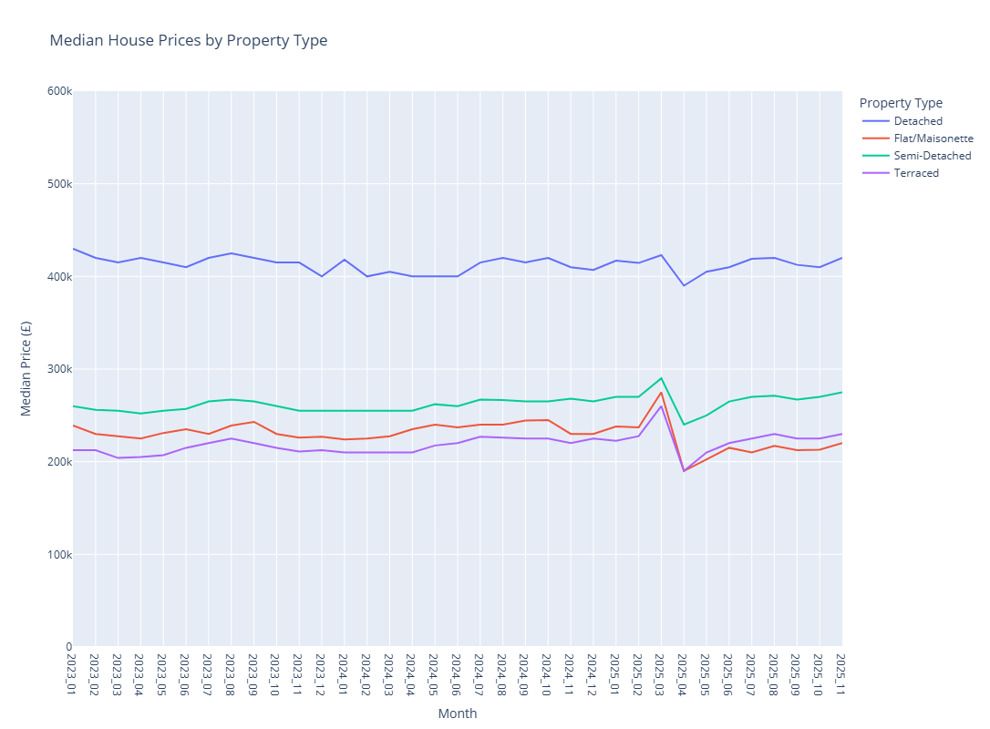
Let's illustrate this by doing generating some analytics in this notebook using the data we have just written to the lakehouse in Delta format.
# Load prices from Delta and filter them to exclude "Other" property types
logger.info(f"Reading prices data back from Delta table: {target_path_prices}")
prices = (
    pl.scan_delta(
        target_path_prices,
        storage_options=storage_options,
    )
    .filter(pl.col("property_type") != "Other")
)
INFO: Reading prices data back from Delta table: ../data/fabric/Tables/house_price_analytics/prices
INFO:notebook_logger:Reading prices data back from Delta table: ../data/fabric/Tables/house_price_analytics/prices
# Load the date dimension, a new month_tag column in the form YYYY_MM
logger.info(f"Reading dates data back from Delta table: {target_path_dates}")
dates = (
    pl.scan_delta(
        target_path_dates,
        storage_options=storage_options,
    )
    .with_columns(
        [
            pl.col("date").dt.strftime("%Y_%m").alias("month_tag")
        ]
    )
)
INFO: Reading dates data back from Delta table: ../data/fabric/Tables/house_price_analytics/dates
INFO:notebook_logger:Reading dates data back from Delta table: ../data/fabric/Tables/house_price_analytics/dates
# Now join the two tables to get month_tag into the prices table
prices = (
    prices
    .join(
        dates.select(
            [
                "date",
                "month_tag"
            ]
        ),
        left_on="date_of_transfer",
        right_on="date",
        how="left"
    )
)
# Finally summarise the data up to monthly level by property type
monthly_summary = (
    prices
    .group_by(
        [
            "month_tag",
            "property_type"
        ]
    )
    .agg(
        [
            pl.len().alias("number_of_transactions"),
            pl.col("price").median().alias("median_price"),
            pl.col("price").min().alias("min_price"),
            pl.col("price").max().alias("max_price"),
        ]
    )
    .sort(
        [
            "month_tag",
            "property_type"
        ]
    )
)
monthly_summary = monthly_summary.collect()
# Plot the monthly summary using Plotly
import plotly.express as px

fig = px.line(
    monthly_summary,
    x="month_tag",
    y="median_price",
    color="property_type",
    title="Median House Prices by Property Type",
    labels={
        "month_tag": "Month",
        "median_price": "Median Price (£)",
        "property_type": "Property Type"
    }
)
fig.update_yaxes(range=[0, 600000])
fig.show()
Performance Optimisation Tips
- Use lazy evaluation for large datasets - for datasets approaching memory limits, lazy evaluation lets Polars optimise the query plan.
- Optimise row groups for DirectLake - if your Delta tables will be consumed by Power BI's DirectLake mode, configure larger rowgroups. See this blog "Delta Lake Tables For Optimal Direct Lake Performance In Fabric Python Notebook" from Sandeep Pawar (Principal Program Manager, Microsoft Fabric CAT) for more details.
- Scale up your notebook environment when needed - using the
%%configuremagic command in a cell at the top of the notebook. Available configurations: 4, 8, 16, 32, or 64 vCores (memory scales proportionally).
Current Limitations
A few things to be aware of:
- V-ORDER - Fabric's V-ORDER optimisation requires Spark; Polars-written Delta tables won't have this applied. Tuning rowgroups can partially compensate.
- Liquid Clustering - similarly, Liquid Clustering is Spark-only.
- Polars version - the pre-installed version may lag behind the latest release. You can upgrade with
%pip install polars --upgrade, though this adds notebook startup time. - Memory ceiling - the maximum single-node configuration is 64 vCores. Beyond that, you'll need Spark or Polars Cloud (when available).
Further reading
- Microsoft Learn: Python experience on Notebook
- Microsoft Learn: Choosing Between Python and PySpark Notebooks
- DeltaLake Documentation: Using Delta Lake with polars
- Sandeep Pawar: Working With Delta Tables in Fabric Python Notebook Using Polars
Summary
Polars on Microsoft Fabric offers a compelling alternative to Spark for many data engineering workloads. The combination of Polars' performance, Fabric's native OneLake integration, and the cost efficiency of single-node compute creates a practical path for teams who want enterprise-grade data pipelines without the complexity of distributed systems.
Start small, measure your workloads, and scale to Spark only when you genuinely need distributed compute. For many teams, that day may never come.
This is Part 4 of our Adventures in Polars series:
- Part 1: Why Polars Matters — The Decision Makers Guide for Polars.
- Part 2: What Makes Polars So Scalable and Fast? — The technical deep-dive: lazy evaluation, query optimisation, parallelism, and the Rust foundation.
- Part 3: Code Examples for Everyday Data Tasks — Hands-on examples showing Polars in action.
Are you running Polars workloads on Microsoft Fabric? Have you found effective patterns for switching between local development and cloud deployment? We'd love to hear about your experiences in the comments below!

