Modern Compute: Unavoidable Practicalities


In this series on modern compute capabilities I will be looking at many aspects of the computational landscape, but there are certain universal truths. In this post, I will describe some of the basic laws of nature that apply to any form of computation. A deep understanding of these truths is essential to choosing the right computational mechanisms for your applications.
These will lead us to a particularly important concept: the threshold of usefulness. Determining where this threshold lies is critical to maximising performance.
You have to get your data to your compute
Even Seymour Cray ran aground on this first truth. Cray was arguably the most successful supercomputer designer our industry has ever seen. His CDC 6600 outperformed its contemporaries by an order of magnitude. The supercomputers he designed at Control Data Corporation, and then the eponymous Cray Research dominated the supercomputing world for over two decades. His Cray 1 demonstrated the incredible potential of vector processing, and the SIMD capabilities of modern CPUs are arguably the result of what Seymour Cray taught us back in the 1970s.
But with the Cray 2, the fastest computer in the world when it was released, Cray's creations had become so fast that this first law of nature began to bite. The Cray 2's theoretical performance was elusive in practice. There were a few reasons the Cray 2 did not enjoy the success of Cray's earlier work, but one of the most important ones was the unavoidable fact that you have to get your data to your compute capacity.

The fastest computer in the world is of little use if it spends almost all of its time waiting for the inputs to the next calculation.
This is even more of a problem today than it was for the Cray 2 back in 1985—raw computational performance has continued to improve more quickly than memory speed. The amount of trouble this causes varies, because the amount of work required for a particular quantity of input data varies from one application to another, but it is a very common constraint on performance.
There are a few scales to consider when thinking about getting your data into a place you can work with it:
- region: you might have terrabytes of data in a factory that is hundreds of miles from the datacentre in which you'd like to process it
- datacentre: your data might be in a data lake in the same cloud provider region as your compute, but given the size of typical cloud computing facilities, they could still be in different buildings, possibly at opposite ends of some industrial estate
- network distance: even in within a single building, the difference in transmission time between the most physically close and the most distant nodes can be large
- compute node: even with the most favourable physical network layout and the most advanced networking systems, getting data from a persistent store into a node where you can run your code is much, much slower than memory access speeds for data already on the machine
- memory hierarchy: even if your data is in the right computer, that doesn't guarantee it'll be available fast enough—the time it takes to get data from main memory into the parts of the CPU that can work with it can be enough time to execute hundreds of instructions
- device-specific memory: your data may be in memory and even in the L1 cache, but if you were hoping to get the GPU to work with it, you've got to copy it to the GPU's memory (possibly flushing the L1 cache out to main memory first)
That last one can explain why even in situations where a GPU or custom ASIC looks like the best candidate for a particular computational job, it might actually be faster in practice to use the CPU. If the data you want to work on happens already to be available high up in the CPU's cache hierarchy, the CPU might be able to complete the work in less time than it would take to copy the data to where the GPU can see it.
Data layout matters
Even if your data is exactly where it needs to be, challenges remain. The way in which data is arranged in memory can have a significant impact on performance. Modern CPUs typically fetch data from main memory in chunks (e.g. 64 bytes), which works well if the values an algorithm needs to process are adjacent in memory.
If you need to process a grid of data (e.g., the pixels in an image) this chunked memory access can mean there is a big difference between working from left to right across a row, and working from top to bottom along a column. We have a choice about how we store a grid of data, and this choice can determine which direction works fastest. Consider this small grid:
| 0A | 1A | 2A | 3A |
| 0B | 1B | 2B | 3B |
| 0C | 1C | 2C | 3C |
| 0D | 1D | 2D | 3D |
This is a 4x4 grid of data, and to help make it easier to keep track of which cell is which, I've used a number to indicate the column and a letter to indicate the row. Computer memory is effectively linear—it's all ultimately just a sequence of bytes. (Memory devices do actually arrange the transistors that store data in a 2D grid, but this implementation detail has no visible consequences for developers.) So a grid like this has to be flattened out into a list. There are two common ways to do this. There is row-major order, in which we store the first row, followed by the second, and so on:
0A, 1A, 2A, 3A, 0B, 1B, 2B, 3B, 0C, 1C, 2C, 3C, 0D, 1D, 2D, 3D
Alternatively, we might use column major order in which we store the first column, then the second, and so on:
0A, 0B, 0C, 0D, 1A, 1B, 1C, 1D, 2A, 2B, 2C, 2D, 3A, 3B, 3C, 3D
Suppose each value in our grid is 8 bytes in size (the size of a double-precision floating point number). Also, to simplify the following discussion, I'm going to presume that the data happens to start at a memory location whose address is an exact multiple of 64, and also that we're using a CPU with a 64-byte cache line size (a common size). If we read the top-left entry of the grid, the CPU will not just load that first entry into the L1 cache. It will fetch 64 bytes of data starting from that location—it will fetch 8 of our 8-byte values. If the data is stored in row-major order, that means it will fetch this data:
0A, 1A, 2A, 3A, 0B, 1B, 2B, 3B
That means the values shown in bold here will be fetched from main memory into the CPU cache:
| 0A | 1A | 2A | 3A |
| 0B | 1B | 2B | 3B |
| 0C | 1C | 2C | 3C |
| 0D | 1D | 2D | 3D |
In other words, the entire first two rows will be loaded. (If the grid were 8 values wide, it would just be the first row. If it were wider still, it would fetch the first 8 values of the first row.)
If our code processes data from left to right, this is great—a single memory access has loaded the entire first row, so no further fetches from main memory will be required as we process the rest of the values in that row. And if we're going from left to right and then from top to bottom, we'll process the whole of the first two rows here with just a single memory access. (Moreover, CPUs typically detect when our code is accessing elements in order like this, and may start fetching subsequent data in anticipation of it being needed, which means that by the time we've finished processing the first 8 values, the next ones we need may already have been loaded.)
But what if our algorithm needed to process the data from top to bottom? (E.g., with the matrix multiplication operations that neural networks use, we need to combine all the values from one row of one matrix with all the values from one column of the other matrix: our algorithm proceeds across each row in turn for one input, and down each column in turn for its other input. So you actually get both directions in a single algorithm in that case.)
For that pattern, the CPU's loading of 64 bytes of data has been less helpful, because it has fetched only half of the first two columns. And if the grid were larger it would be worse. If each row is longer than 64 bytes, each fetch from the row-major format would read just one value from the column we want, and 7 values we don't care about, instead of fetching the next 8 values that we'll need to process. So when an algorithm proceeds initially from top to bottom (and then left to right for each column), the column-major layout works better on modern CPUs. With that layout, the first read would fetch these values:
0A, 0B, 0C, 0D, 1A, 1B, 1C, 1D
On the grid, that's the values in bold here:
| 0A | 1A | 2A | 3A |
| 0B | 1B | 2B | 3B |
| 0C | 1C | 2C | 3C |
| 0D | 1D | 2D | 3D |
If our processing wants to look first at every value in the first column, and then every value in the next and so on, this has clearly worked out better than the row-major order. But obviously this layout is suboptimal for processing that wants to look at the whole of the first row, then the second, and so on. In fact, this example suggests that for matrix multiplication, where we want to look at one matrix row by row, and the other column by column, that it would be optimal to use row-major order on one of the inputs, and column-major order on the other!
With GPUs it gets a good deal more complicated because those are able to coalesce memory accesses performed across quite large numbers of threads. In small examples like this, that might actually simplify things. As long as your data does not exceed a certain size, the GPU might in fact be able to fetch all data required into the cache in a way that is optimal even though the layout appears not to be helpful. However, for problems large enough to be worth sending to the GPU, layout in memory still tends to be very important.
It's not unusual for high-volume number crunching code to spend a non-trivial amount of time re-arranging data in memory to enable the main computation to proceed more quickly.
You have to get your results out
It's not enough to perform a computation. You must deliver the results to where they are needed. If the task is to decode a video stream, we probably want the results to appear on screen, which means they need to be in the memory used by the graphics hardware. If we are performing statistical aggregation over very large data sets as part of an analytics data pipeline, the final results are probably going to be written to a data lake, which means that once computation is complete, we will need the data to reside somewhere in the computer's main memory, so that the networking hardware can send that data to the lake.
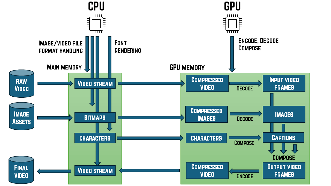
Sometimes, there might be quite complex sequencing and orchestration. In video production, we might be decoding one video stream to incorporate it into another video stream as output. In this case, the final destination might actually be an mp4 file on disk, but the whole process would typically entail decoding the input video, possibly performing some image processing, or mixing in other imagery such as captions or visual effects, and then encoding the results into a new video stream. And in this case, the encoding of that final output stream is probably going to be done on the GPU, so even in this case, where the final destination is a storage device, the decoding of the input video needs to be done to GPU memory even though that particular video stream probably isn't going to be displayed on screen.
But no matter how simple or complex the processing structure may be, getting the output where we need it to be can often be a significant part of the overall cost. As with the earlier problem of getting inputs to where the computational capacity can reach it, these equivalent considerations on the output side may also mean that an apparently optimal choice of computation mechanism might not be the best choice in practice: again, the costs of moving the data might matter more than the performance improvements we might get by using the most capable hardware.
In an extreme case you might determine that some 5-stage process happens to do work where stages 1, 3, and 5 are very well suited to the GPU, but stages 2 and 4 would be more efficiently handled by the CPU. The costs of moving data back and forth between the CPU and GPU might mean it makes more sense to chose a suboptimal location for one or more of the tasks to reduce the amount of data movement.
The threshold of usefulness
The issues described in the preceding sections point to an important idea: the threshold of usefulness. When considering whether to use specialized computational capacity (e.g., an NPU or a GPU), or a high-volume architecture such as Spark, there will always be some problems that are too small to be worth the trouble.
It will, I hope, be obvious that there's no sense in firing up a Spark cluster to evaluate the sum 2 + 2. But this raises the question: what kind and size of problem does justify the use of Spark? Or an NPU? Or a GPU?

There are two important facets to this question.
First, how well does the computation mechanism you're thinking of using fit the problem you've got? Some problems are very well suited to a GPU, for example, but some are not. So any time you have data in one particular place (e.g., main memory) and you're thinking of moving it to another place (e.g., the GPU's memory, or perhaps the main memory of a different machine in your Spark cluster) you should only consider doing so if there's a good reason to think that this offers some inherent computational advantage over processing the data wherever it happens to be right now.
Second, even if the work is a particularly good fit for the compute capacity you're thinking of moving the data to, you need to work out whether the benefits will outweigh the costs of moving the data. There are a few factors that might affect this determination; the volume of data being processed is the most common one, but there may be others such as the amount of work you need to do on the data, but for the present purposes, we can describe all relevant factors as, in some sense, the size of the problem.
The threshold of usefulness is the problem size at which it becomes worth moving the data to take advantage of computational capacity that is a better fit for the data than the capabilities available wherever the data happens to be right now. E.g., an NPU is much faster at matrix multiplication than a CPU, but if you only need to multiply a single 2D vector by a 2x2 matrix, that will be below the threshold of usefulness.
Data dependencies limit parallelism
All of the various options for computation in this series (aside from the default: vanilla single-threaded code running on a single CPU) speed things up through some form of parallelism. Up until about 25 years ago, Moore's law went hand in hand with single-threaded performance improvements. Each new generation of computers essentially did what the previous generation did1 but twice as fast. Unfortunately, that ground to a halt shortly after the turn of the century, and the majority of the improvement since then has been in the form of ever-increasing amounts of parallel computing capacity. Moore's law—doubling the transistor count every 2 years—still applies, but those transistors stopped doubling their speed over two decades ago.
To draw an analogy, if the automotive world had progressed as quickly as computer performance did up until about 2003, each new car model would have had a top speed that was double that of its predecessor, with equally impressive improvements in acceleration, braking, and cornering capability. But things changed round about 2003. Since then, outright speed and handling would have improved only slightly, but every new model would have had twice as much space in the trunk. For certain use cases, an 18-wheel semi-trailer is faster than a Ferrari, and this is the specific kind of speed Moore's law has mostly been delivering for the last two decades. The improvements in flat-out speed may be modest, but the sheer quantity that we can shift has increased vastly.
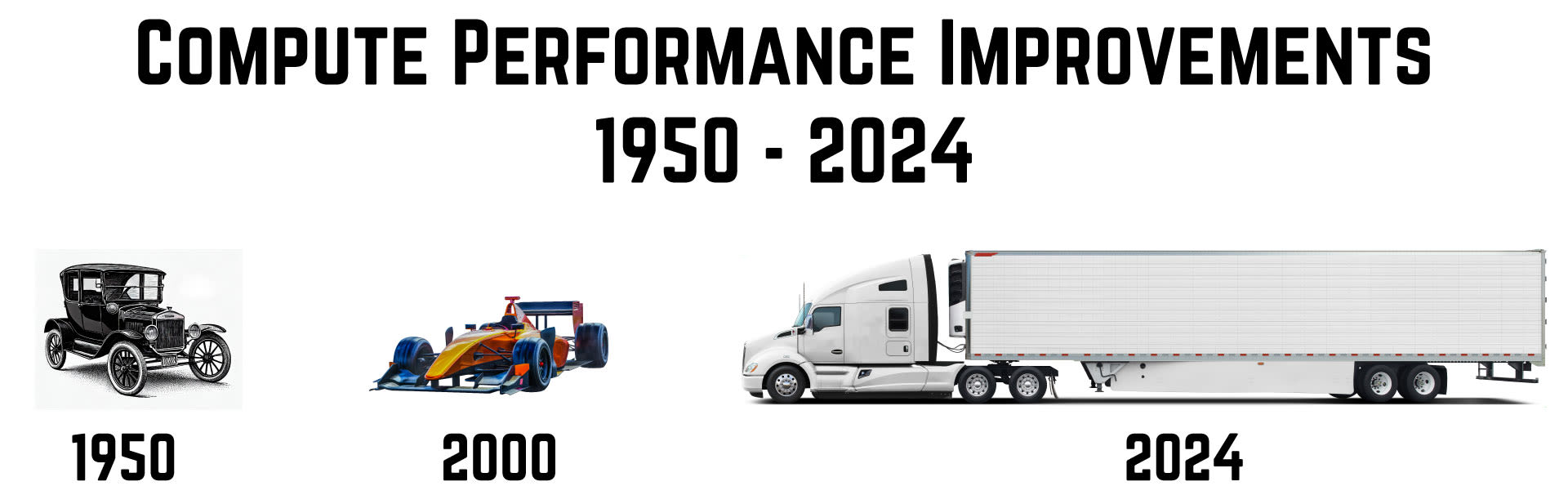
The snag is that all the additional power Moore's law has given us is of no use for certain problems. A massive truck hauling a storage container is not an efficient way to deliver a single, small package. This is why the phrase "embarrassingly parallel problem" often gets used when talking about modern computational capacity, especially GPUs: just as a huge delivery vehicle is good at shipping thousands of identical packages to the same place at the same time, GPUs are good at performing an identical sequence of calculations across thousands of inputs all at the same time. A CPU or sports car might process or move an individual input or package faster, but if you want to do exactly the same job with thousands of things, the more ponderous GPU or truck will perform better overall because it can handle so much at once.
The flip side of this is that if the problem you need to solve is not amenable to parallel processing, you won't get any benefit from a GPU. (Or an NPU for that matter. Those also deliver their power through parallelism.)
Why might a problem not be amenable to parallel processing? Why can't we always just divide and conquer, splitting the work into thousands of individual steps, and performing all of those steps simultaneously?
In a word: dependencies.
If step 2 of a calculation depends on the results of step 1, I can't begin step 2 until step 1 completes, meaning that I can't perform these two steps concurrently. Almost all of the work we get computers to do has some dependencies of this kind. Even with the kinds of problems often described as "embarrassingly parallel" there is usually some kind of flow of information through the system.
The computer scientist Gene Amdahl showed (back in 1967) that dependencies impose a limit on the extent to which parallelism can help us. Amdahl's law is actually more general, demonstrating that optimizing any single part of the system inevitably reaches a point of diminishing returns, but it is often cited in the context of parallel processing. He showed that in a problem where 95% of the computational work can proceed in parallel, parallelism will never deliver move than a x20 speedup no matter how many CPUs you throw at the problem.
Since Moore's law has, for the last 20 years, been delivering higher performance mostly in the form of increased parallelism, that's a crucially important point. The exponential improvements that Moore's law seems to offer are often impossible to exploit in practice.
One of the reasons neural networks have seen a resurgence in interest in recent years is that they happen to have a very high proportion of parallelisable work. There are still some dependencies—we have to calculate the weighted sum of all of the inputs to a particular neuron before feeding that into the activation function for example, and we can't start work on any particular neuron layer until all of its inputs are available. But even so, the proportion of parallelisable work is very high, making this one of the few workloads that can fully exploit as much parallel computational capacity as current computers are able to supply.
To pick an example from the opposite end of this parallelisability spectrum, we can look at the kind of work most cryptographic algorithms do when we're using them to protect our data. (Attacking cryptosystems is another matter; parallelism does help there because if you're simply trying to guess a password, the ability to try thousands of guesses concurrently definitely does speed up an attack.) Many encryption and hashing algorithms perform a series of steps where the output of each step feeds into the next, making them almost entirely unparallelizable.
Business logic often has sequential elements because it might involve "if this, then that" rules. Causality is often part of what's being expressed.
Sometimes apparently sequential logic can, through clever manipulation, be converted into something more readily parallelizable. Or there may be parallelizable heuristics that don't give precisely the answer you want, but which are close enough to be acceptable if they can be produced more quickly or at lower cost.
You can't just "write once, run everywhere"
This series of articles has been motivated by innovation in hardware—we have access to computational mechanisms that were not widely available a few years ago. This comes hand in hand with diversity of technology. This is good insofar as it means that many different possibilities are being explored, increasing the chances of valuable new techniques being discovered. But one significant downside is that software that takes advantage of this can end up only being able to run in very specialized computing environments.
For example, although SIMD support is now more or less ubiquitous in modern CPUs, the exact feature set varies quite a bit from one processor kind to another. So although you can pretty much count on being able to execute addition and multiplication on 4 floating point point numbers held in a 128-bit vector register on any modern CPU, you might not be able to count on certain more rarefied operations. For example, some CPUs offer vectorised bit counting (i.e., counting how many of the binary digits in a number are non-zero, and doing this simultaneously for all 16 bytes held in a 128-bit vector register), but many do not.
NVidia's CUDA system is a very popular way to exploit the computational capabilities of GPUs, but code written for CUDA won't work on AMD's graphics cards. (You might be able to use something like SCALE to get CUDA code working on an AMD device, but getting any kind of commercial support for this might be tricky.)
Microsoft's Direct3D (and for computational work, the DirectML feature in particular) provides a layer of GPU vendor independence, but this then ties you to Windows.
Vulcan is an attempt to provide a unified API over Nvidia, AMD, Apple, and Intel hardware, but it can't currently drive some NPUs. WebGPU is a similar idea, available only inside of a web browsers.
There are numerous options that look at first glance like they might provide some level of hardware agnosticism. Besides Vulcan, there are ONNX, Tensorflow, and PyTorch, for example. However, although each of these can run on a range of hardware, in practice none of them covers everything. There are gaps in the coverage of pretty much everything at the moment.
Summary
So those are the basic laws. Getting data to and from the computational machinery has its costs. Dependencies in our data may limit the potential for performance improvements. And every toolset for using the more exotic modern compute hardware has incomplete coverage. As you'll see in the remainder of this series, these concerns all crop up a lot.
In the next entry in this series, I will look in more detail at some of the kinds of workloads that might be able to take advantage of modern computational capabilities.
-
to be strictly accurate, new CPU generations often provided more than just a speed boost. Intel's main CPUs have increased both the number and size of their registers over time. However, that was arguably necessitated by the improvements in performance: as power increased, CPUs were able to tackle larger and larger problems, meaning we wanted more memory, something Moore's law provides, but that meant we needed to move from 16-bit to 32-bit and then 64-bit architectures to be able to address ever increasing volumes of data. But even when new generations of CPUs added new features, it was also true that up until about 25 years ago, if you only used your new CPU to do all the things your previous CPU could do, it would do it roughly twice as fast if you upgraded every 18 months.↩