Evaluation Contexts in DAX - Relationships


TLDR; After learning about the two different types of evaluation contexts in our previous post, we now talk about table relationships and how these interact with the filter and row contexts to condition the output of our DAX code.
In our previous article on Evaluation Contexts in DAX, we learned about the two types of evaluation contexts, namely the filter and row contexts – and how these dictate how any formulas that we write in DAX are calculated. There is one further key aspect to take into account when understanding how our results are calculated – relationships. Most data models, like the ones we use to visualise data in Power BI reports, are composed of many data tables. These data tables are connected with each other through relationships. In this post, we will see the different types of relationships and how these affect the output of our DAX code.
Table relationships
Let's reuse the example from our previous post. Say we have a data model containing data on the sales of certain products from a store. We have a “Sales” table containing the details of each sale made and a “Product” table, containing details about the products available in the store, amongst others. The Sales and Product tables are clearly related to each other, since the Sales table tells us which products where sold, and the Product table gives information about the products themselves, like their colour, brand, and price.
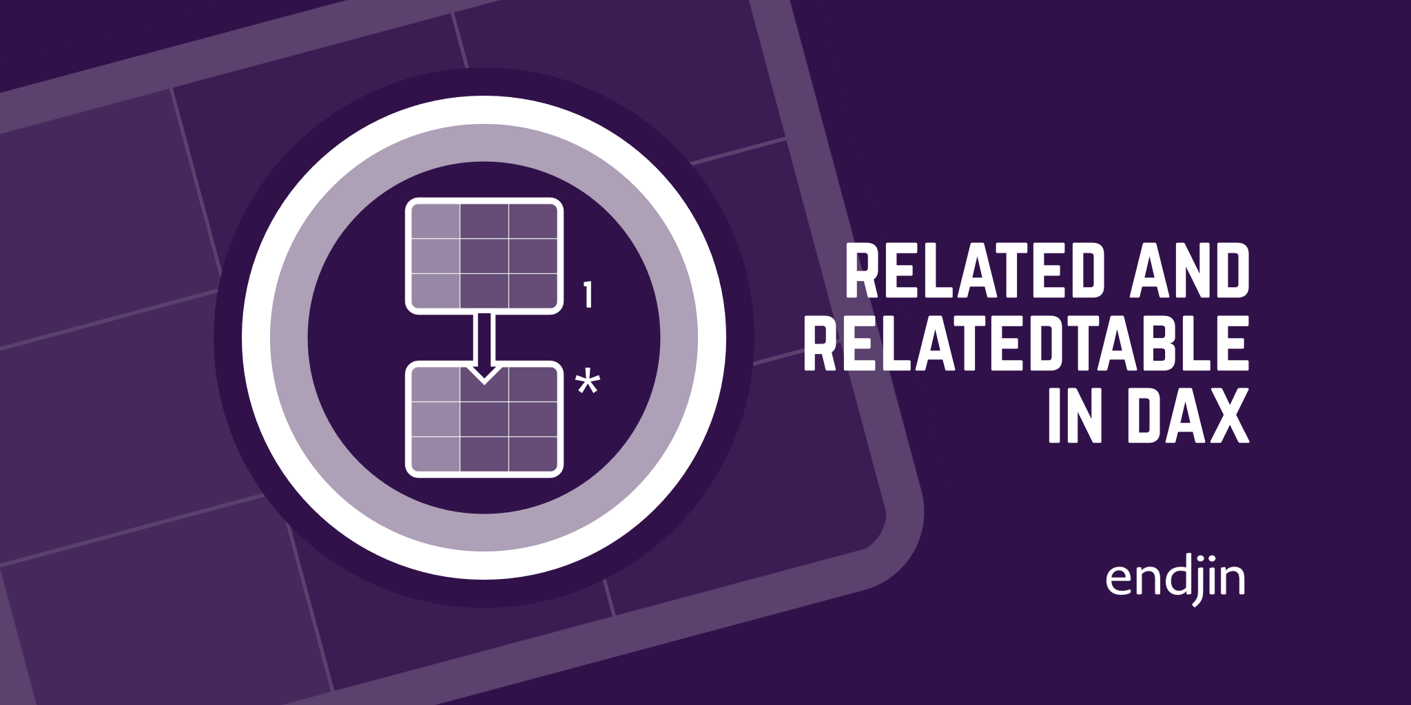
Relationships have a direction and two sides.

The direction of the relationship dictates how Power BI will apply filters from one table to another, meaning which table is allowed to filter the other. The relationships can be either unidirectional or bidirectional. It is standard practice to keep relationships unidirectional wherever possible, since bidirectional relationships are harder to predict.
The sides can be either the “one” side or the “many” side. One same product can be sold many times, so it can feature more than once in the Sales table. Hence in this relationship, the Product table is on the one side, and the Sales table on the many side. It is possible to have many to many relationships, but these make the data model more complex. When we look at the data model in Power BI, the one side is denoted by a “1”, and the many side is denoted by an “*” sign. The direction of the relationship is shown by an arrow pointing to either or both tables.

Now that we have seen how tables can be related to one another, let's look at how these relationships affect our evaluation context.
Row Context
Understanding how the row context affects relationships is easy, because it doesn't. The row context is not propagated through relationships, hence why Power BI doesn't allow the creation of calculated columns computed from two or more different tables.
In order to propagate the row context from table to table, we need to use the RELATED and RELATEDTABLE functions.
RELATED function
The RELATED function is used to force the row context to propagate from the many side to the one side. The row context iterates through the table on the many side, and finds the one corresponding row on the table on the one side.

Imagine we want to add a column in our Sales table that indicates the color of each sale made. The color is specified in the Product table, which is on the one side of the one to many relationship with the Sales table.
If we simply indicate that we want our new column to be equal to the color column in the Product table, we get an error.
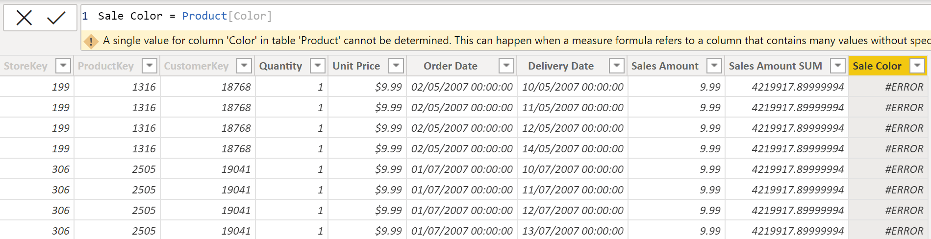
A single value for column 'Color' in Product table cannot be determined because the row context hasn't been propagated from the Sales table (the many side) to the Product table (the one side).
By using the RELATED function, the row context is correctly propagated.

RELATEDTABLE function
The RELATEDTABLE function is used to force the row context to propagate in the opposite direction, from the one side to the many side. Here, because the row context iterates through the table on the one side, it will find many corresponding rows on the table on the many side, which RELATED would identify as an error. RELATEDTABLE will return all rows found on the many side when the row context is applied on the one side.

Here, the filter context from the Product table is being propagated to the Sales table, finding many matches. Finally, the sum of the quantity of all sales for each item is computed.
Filter Context
The filter context does propagate through (some) relationships, but only from the one side to the many side. Bidirectional relationships need to be activated for the propagation to happen the other way around.
In our example, the product table is on the one side, hence any filters applied on it will propagate to the Sales table, which is on the many side.
Let's illustrate this by filtering a table that shows the quantity of items sold by their color. The color was specified in the Product table, and, in our example above, we created a calculated column for the colour of the items sold in the Sales table using the RELATED function. We will see how the two filters behave differently.
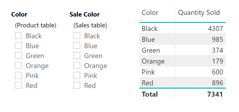
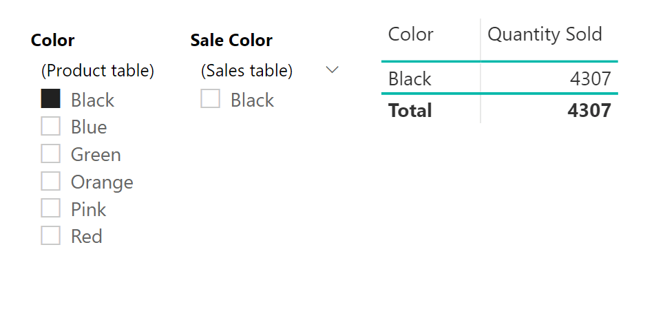
Selecting “Black” in the color filter from the Product table filters our table leaving only one row with the quantity of black items sold. Even our second filter, corresponding to the colour column in the Sales table is filtered out. This works because the filter changes the filter context in the Product table (on the one side) and this is propagated to the Sales table (on the many side).
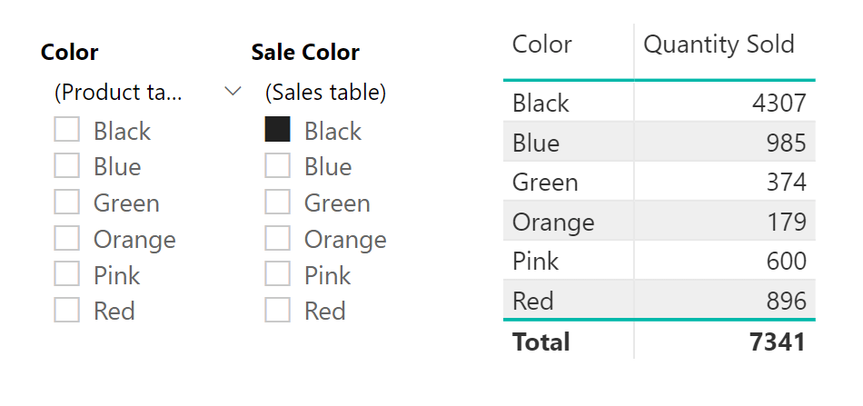
However, selecting black in the colour filter from the Sales table doesn't change our table, which still shows all colors. This is because the filter context on the Sales table (on the many side of the relationship) does not propagate to the Product table (on the one side of the relationship).
Conclusion
We have defined relationships in a data model and how evaluation contexts interact with them. It is important to remember that the row context does not propagate through relationships unless we explicitly state it in our DAX code using RELATED or RELATEDTABLE. Filter contexts, on the other hand, do propagate between tables, always going from the one side to the many side.