Learning DAX and Power BI – Table Functions
So we've looked at the different evaluation contexts, and an overview of aggregator functions, next on the list is table functions!
Table functions are ones that return… A table!
These include:
FILTERALLVALUESDISTINCTRELATED TABLE
A quick reminder of the current state of the dataset we are working with:
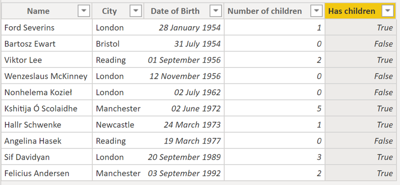
We have a dataset of people who live in different cities, who have different numbers of children and we have created a calculated column to signify whether or not each person has children.
FILTER
The FILTER function does exactly what it says on the tin. You apply it to a table, pass it a condition, and it returns you a "calculated table", which is a filtered version of the table you provided.
For example:
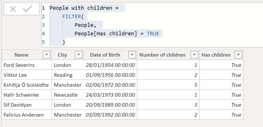
This creates a table which just includes the people who have children. However, this adds another table into the model, which as we've seen means that the report will use more memory on disk.
Instead, if we wanted to do something with this table, we could instead just temporarily store it whilst doing the calculation we require. For example, if we wanted to calculate the average number of children, but ignore those who didn't have children at all, we could do:

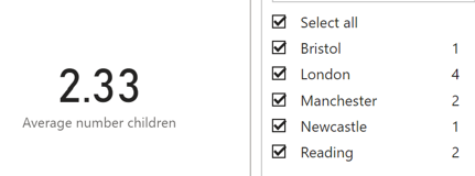
This will give us an average of 2.33, whereas if we include those without children it brings the average down to 2.00.
We can see here that we have defined a variable inside the processing. This becomes incredibly valuable as we build up more complex processing to make the calculations a lot more readable. (We also must use the X-aggregator operators here because the simple aggregators expect a base table as an input.)
We can see that by using this technique we can perform aggregate operations over a conditional subset of the data.
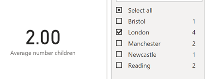
Again, I want to emphasise that this works within the filter context that is applied. E.g. if we applied a page filter so that we were only showing the people who live in London, then the average number of children will change as we have changed the filter context:
DISTINCT
The DISTINCT operator just returns all the distinct values in a column.
For example:
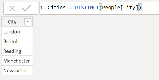
This can be very powerful when building up transformations.
We can also use it combined with COUNTROWS to calculate the number of distinct values in a table:

This will count the number of distinct names there are in the table. We can then apply this measure to find how many distinct people there are in each city:
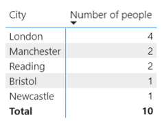
For each row of this table, a filter context of e.g. People[City] = "London" has been applied.
ALL
The next table function is the ALL function. ALL is special in that it ignores all filter context. If you use ALL it will always work over the whole dataset, no matter what external filters have been applied.
This can be useful for calculating percentages/ratios.
Say that you created a measure to calculate the percentage of the people that live in London:

When there are no filters applied you get:
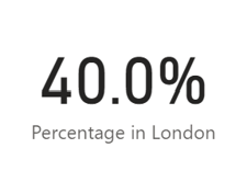
(We can format this as a percentage when we create the measure).
However, if we apply a page filter so that we only show people who are in, say, Bristol, we get:

Because the measure is now operating over a dataset which is filtered to just those who live in Bristol.
But if we add ALL to the table references:

Then the percentage will always show 40.0% because the calculation will ignore any applied filter context and always use the entire dataset.
The ALL operator can also be used to display all the distinct values in a column, regardless of the filter context.
For example:

This is similar to the functionality of DISTINCT, but it will ignore any applied filter context. Therefore, in this case it will always return all of the distinct people in the table.
So, using this:
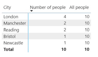
We can see that for the column created by the DISTINCT operator, each cell has scanned the dataset which is defined by the filter context and returned the total number of rows. Whereas for the column which uses the ALL operator, all filter context is ignored and the total number of rows in the whole dataset (10) is always returned.
The final table operator I want to talk about is RELATEDTABLE, but that involves introducing a few new concepts… So, we shall save that for next time!


