Demystifying machine learning using neural networks
A couple of weeks ago I had the opportunity to attend NDC in Oslo. It was an absolutely brilliant experience, and my head is still reeling a bit from everything I learnt! The focus of a lot of the talks was around neural networks and machine learning – something which we have explored quite a lot here at endjin but has always seemed something of a "black box", but no more!
Here I'm going to try and give a quick(ish) overview of what I learnt, and hopefully help to explain exactly what's happening inside those boxes... [WARNING: Some algebra to follow]
Neurons
Neural networks are built up of neurons. In a shallow neural network we have an input layer, a "hidden" layer of neurons, and an output layer. For deep learning, there is simply more hidden layers which allows for combining neuron's inputs and outputs to build up a more detailed picture.
Each neuron can be represented as follows:
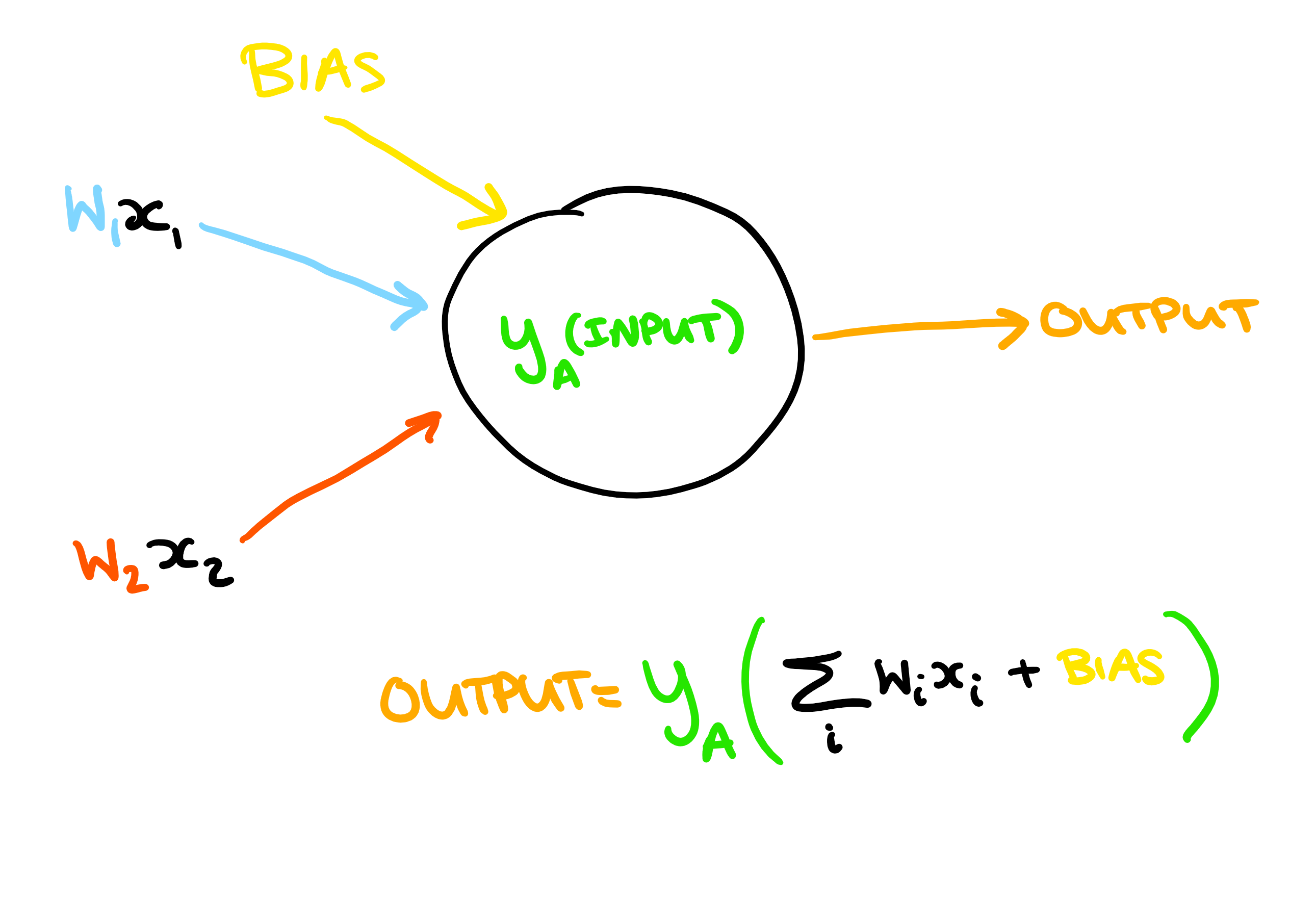
It takes some number of inputs (in this case two), each with a weight, and combines this with a bias. A function is then applied to the total input, to produce an output.

The function that is applied to the total input is called an activation function. This activation function takes our weighted input and produces the output. If we were training a classification model (one which predicts whether or not an input is any of a list of outcomes), you could imagine having one neuron per outcome. When you put an input in, you want the neuron which represents the desired outcome to be as close to 100% activated as possible, and the remaining neurons to remain inactive.
The need for this binary result would seem to imply that a step function would be a good choice. However, if we choose a function which is always either completely "off" or "on", then it is much harder to "learn". At any point, you are either 100% right or 100% wrong. We need the ability to tweak the input parameters to be "more right" as we train the model.
A linear function is the next simplest choice, however using a linear function means that combining layers of neural nets is pointless. This is because the combination of multiple linear functions is still a linear function, therefore the same result could be achieved with just one layer. So for deep learning (with more than one layer of neurons) we require a non-linear activation function.
Activation functions
Here are a few commonly used as activation functions:
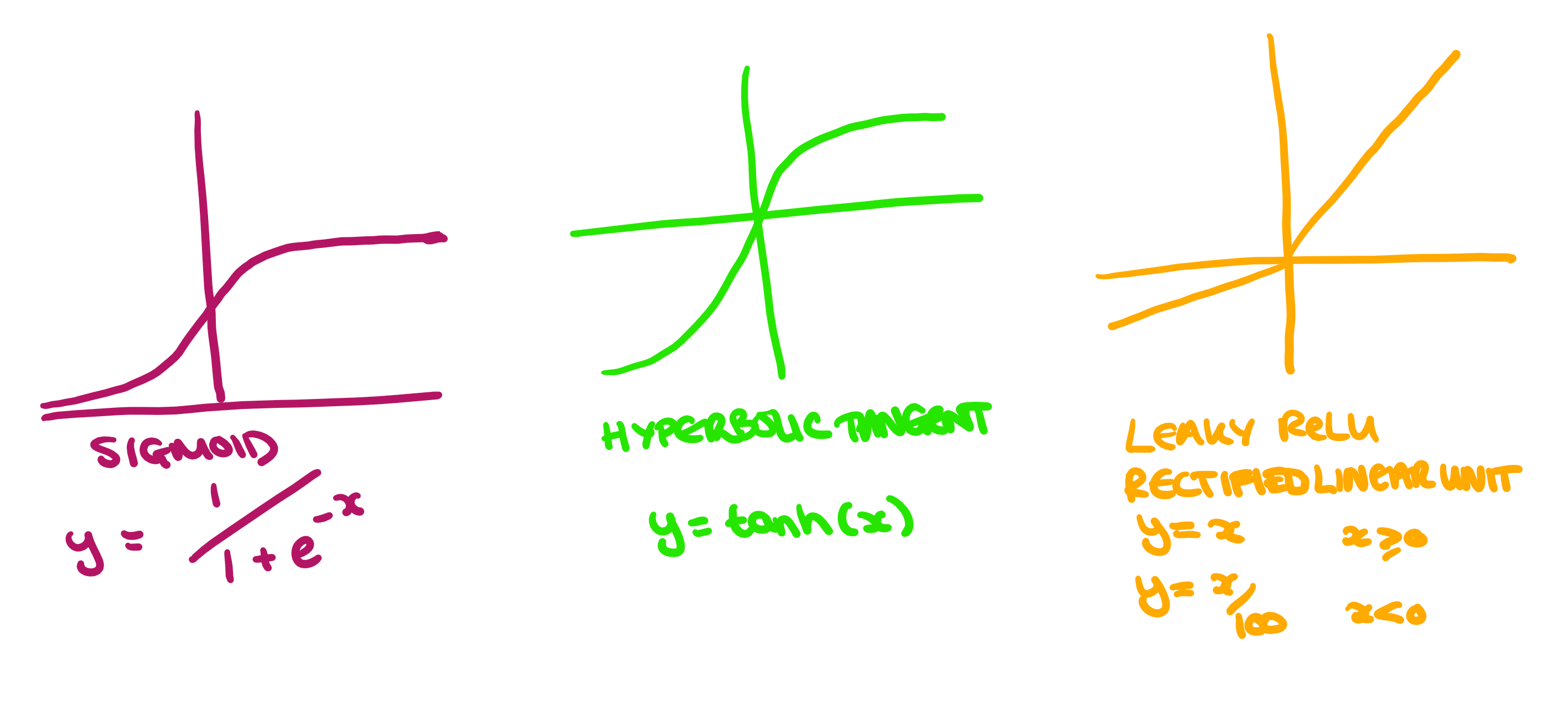
The sigmoid and hyperbolic tangent function (which is really just a scaled sigmoid) are very commonly used in classification networks. They are effective because they have a large gradient in the center, meaning that making small changes in the input will cause the function to move a large amount towards either of the extremes. This is good for classification, where we want an either "yes" or "no" result.
However, the issue with these functions is that when the output is close to the desired value, learning becomes very slow. This means that while it is easy to get close to the result, getting a high degree of accuracy can be difficult/expensive.
These days, by far the most commonly used activation function is a leaky ReLU function. Although it is linear above and below x=0, the non-linearity of the total function means that the combination is also non-linear. It turns out that any function can be approximated by some combination of ReLU functions.
Also note that all these functions only ever increase/decrease. This is desirable in an activation function because if there are points on the curve where the gradient tends to zero, then the algorithm can end up centering on those points.
The final condition for the activation function is that it needs to be differentiable (we'll see why later!).
Neural networks
So, when we first initialize the neurons, we give each of the weights and biases a small random number. For a given input, this might produce the following result (this is an oversimplified picture, as with image classification, you have multiple inputs, which then activate different parts of the hidden layer to produce a combined classification. But I think representing it simply first makes it easier to understand.):
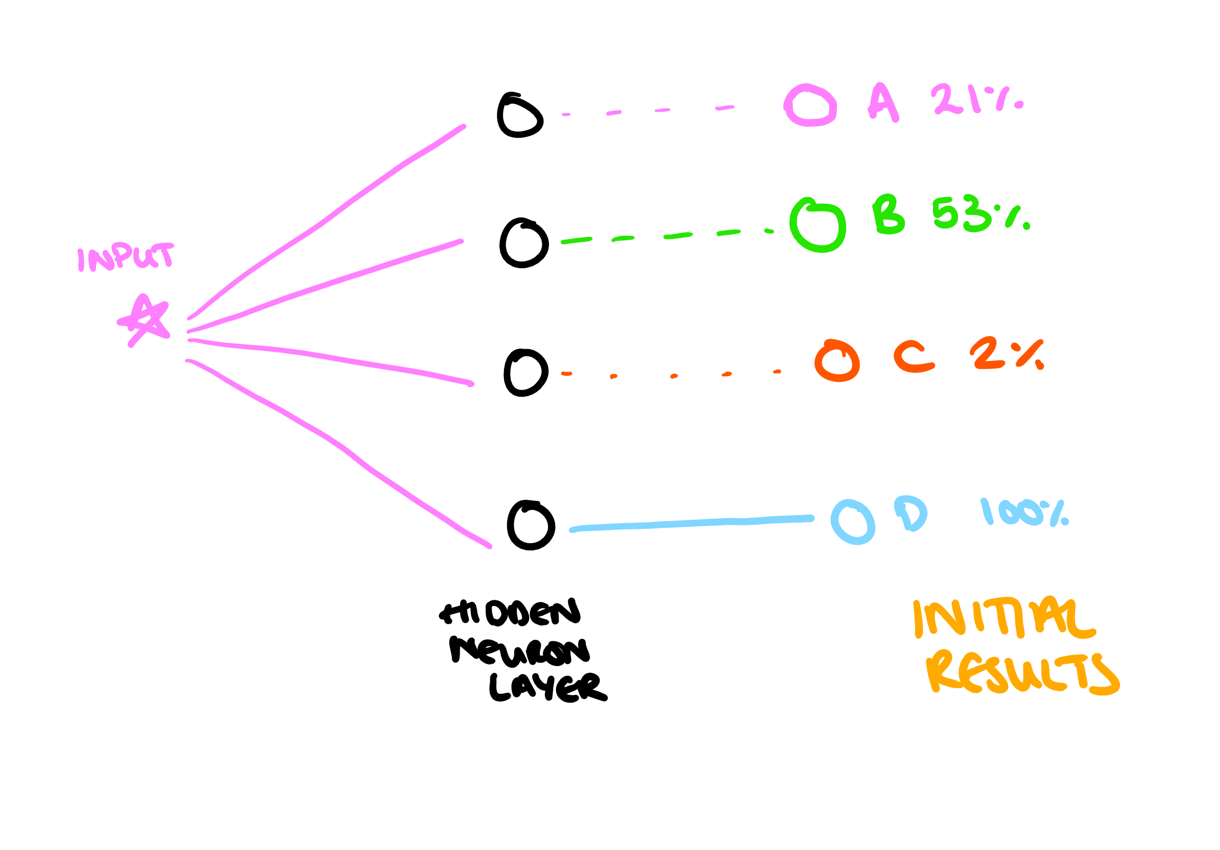
The percentages shown here are the probability that the input "is" in each of the categories. These are completely independent of one another and don't need to sum to 100%. The target result is 100% for A, and then 0% for B, C and D. So we would look at the error in each of these results, and adjust the weights on the input neurons to make the output "a little bit more right". Eventually we might achieve something like this:
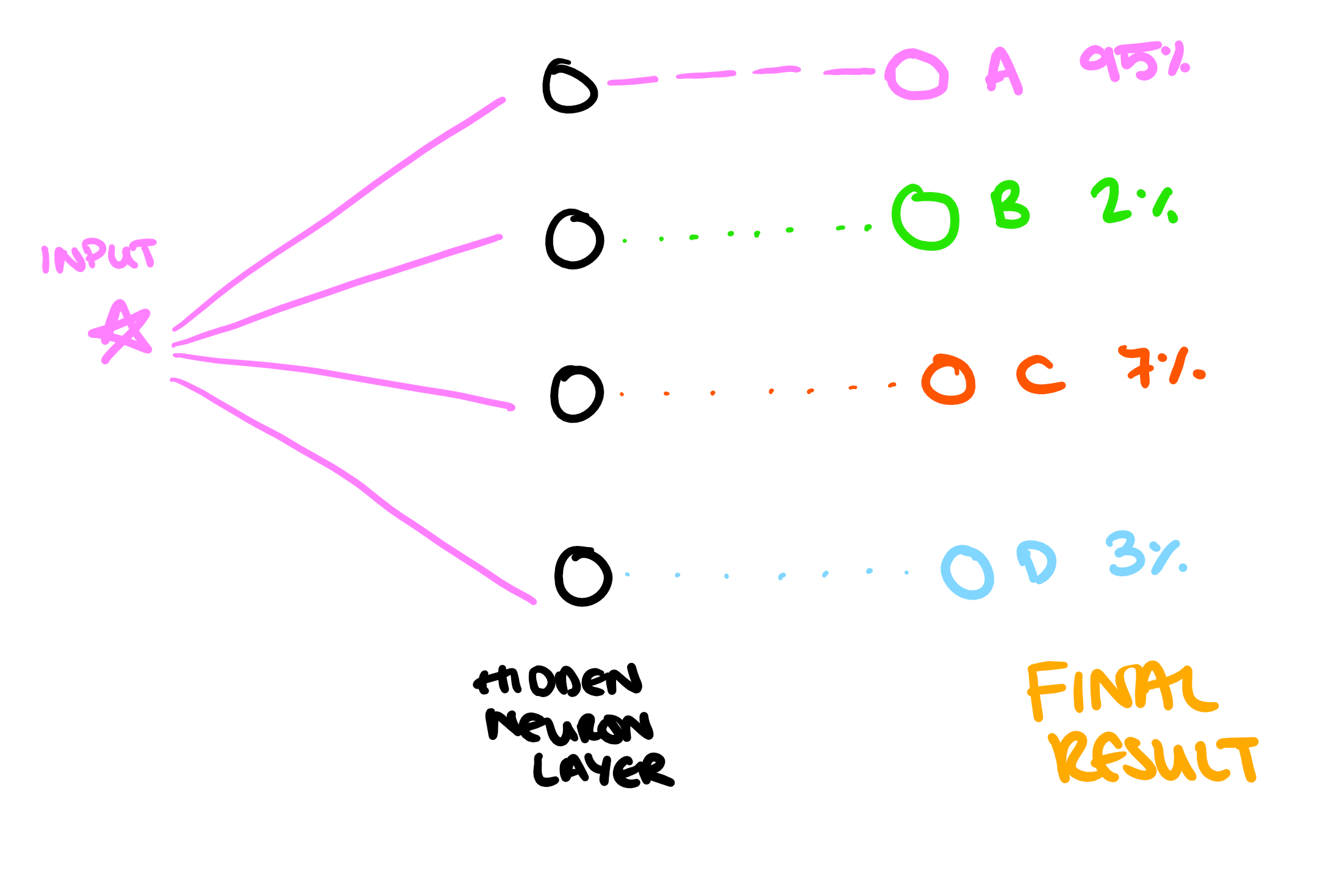
We would also run this through with a variety of different inputs, to train the model to recognise images that should lead to each of the different outcomes.
In reality an image classifier looks something more like this:
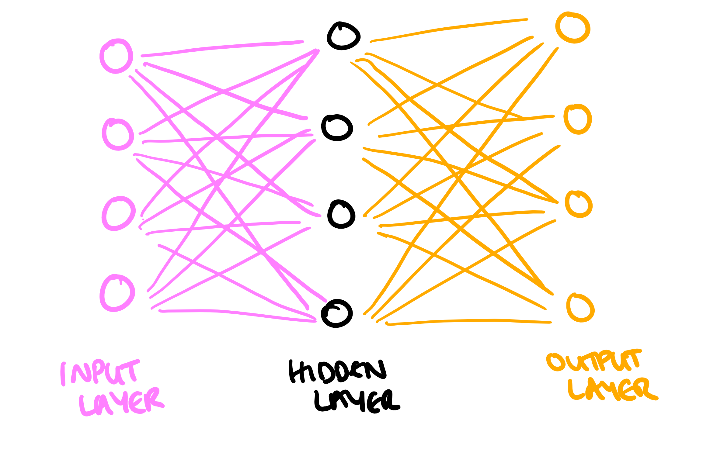
With a different combination of inputs activating each neuron in the hidden layer a different amount, which will then produce a different output (there's a really good visualization of this here!). The difference between shallow and deep learning is just adding more hidden layers, which are all trained using the same process, but allow for a greater and more accurate combination of non-linear functions.
I've mentioned that when the network is trained, the weights and biases are adjusted to make the result "a little bit more right", but how is this achieved?
Training the network
Machine learning via back-propagation uses gradient descent to minimize the error in the output. Gradient descent is an optimization algorithm which essentially means that we want to change the weights proportionally to the gradient of the error with respect to the weight. So, in order to work out how much to change the weight by, we need to work out that gradient (in this example I am assuming one input, one neuron and one output). Here we are using the mean squared formula for the error (E):
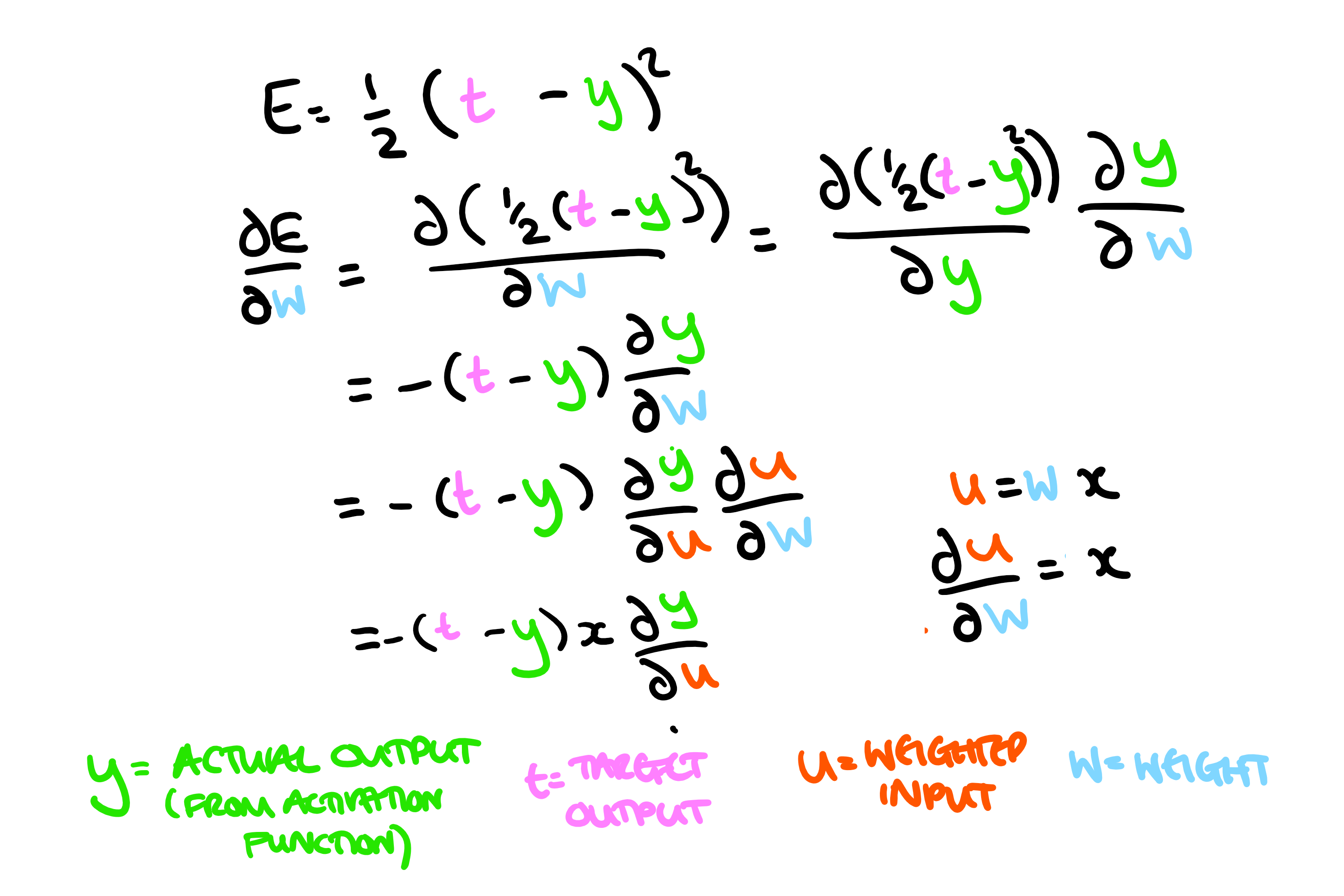
And we want to change the weight proportionally to this gradient, so we have:
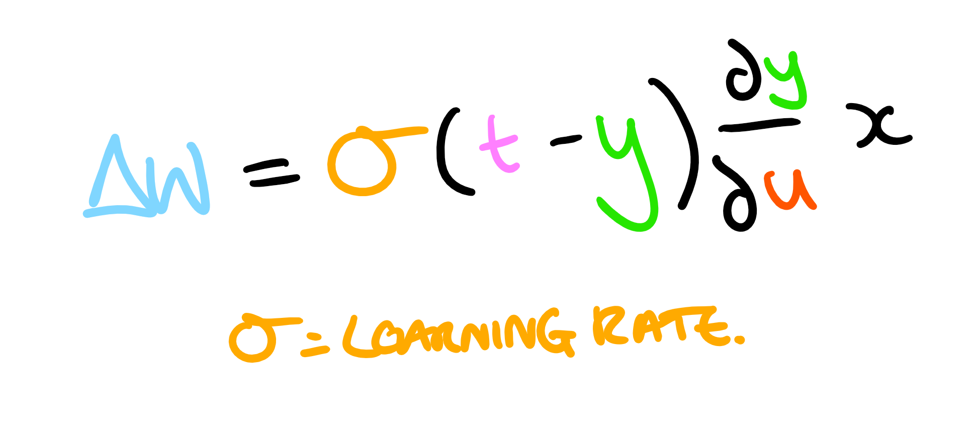
Here we have eliminated the minus (because we want to reduce the error), and the learning rate is the proportionality constant. If we have a higher proportionality constant, then the weight change will be larger on each run through and it will "learn" faster. However, making too large steps leads to larger inaccuracy in the algorithm. The bias is also adjusted for each input. Conceptually, the bias can be thought of as a neuron with a fixed weight of 1. Therefore, at each stage the bias is just changed by the learning rate multiplied by the difference in outputs.
So, for each input the output is calculated. The difference between this and the desired output is then multiplied by the learning rate, the input, and the gradient of the activation function (hence the need for it to be differentiable, and also why if you have points where the gradient is zero the algorithm can get "stuck"). The weight is then changed by this amount, and slowly the total error is reduced.
If each piece of training data is made up of a set of inputs (remember our first neuron with two different x values), which each have an individual weight, this would look something like this:
for (int i= 0; i < numberOfInputs)
{
    weights[i] += learningRate * (targetOutput - realOutput) * GetDifferential(inputs[i]) * inputs[i];
}
All of the inputs' weights are adjusted for a given piece of training data. At the end of a single run through of all the training data (called an epoch) each neuron will have a set of weights which have been adjusted using each set of inputs. Once that is finished, the data is then run through again (known as a second epoch). This further refines the algorithm. This is repeated until a reasonable level of accuracy is obtained. This accuracy is measured against a testing dataset which is not the same as the data used to train the algorithm. This is important because we need to check that the algorithm is able to recognise data it hasn't already seen. Running too many epochs against the same training data can lead to over-fitting of the algorithm to the specific data supplied.
In conclusion...
So the final outcome is a trained neural network (which is really just a load of mathematical functions with tuned parameters), which can evaluate a bunch of inputs it hasn't seen before (so long as they are adequately similar to the data it was trained on) and produce a desired output!
I hope this has somewhat helped to demystify what happens inside a neural network! If you still want to know more, I recommend watching this talk around building up a neural network from scratch, it's a brilliant talk and leaves you with some real-life code to explore!
