RELATED and RELATEDTABLE in DAX

There are multiple functions that can help when you are working with tables that are connected through relationships. RELATED and RELATEDTABLE are two functions that are useful to navigate through relationships when you're working with the row context.

One-to-many relationships

Before we delve into how RELATED and RELATEDTABLE operate, it is first important to understand how one-to-many relationships work in Power BI.

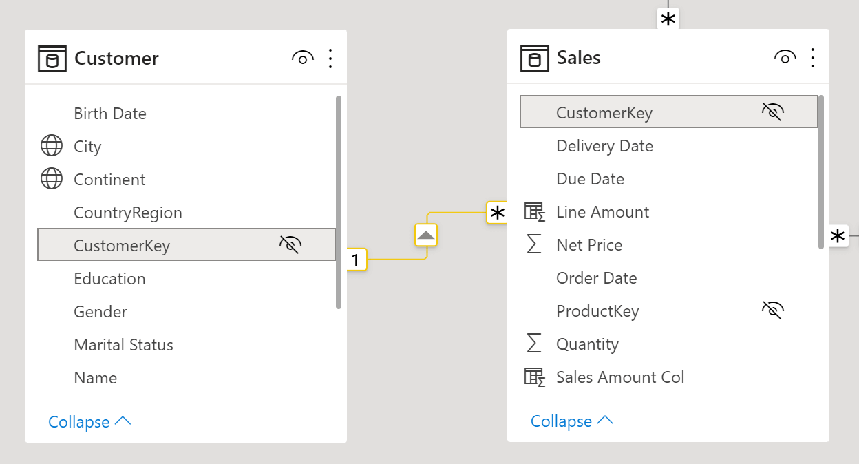
If we take a look at the relationship between the 'Customer' table and the 'Sales' table, we can see that there are two sides of the relationship - a one-side and a many-side. The 'Customer' table is on the one-side (denoted by a 1) and the 'Sales' table is on the many-side (denoted by a *).

In a one-to-many relationship, one row in the table on the one-side can be associated with many rows in the table on the many-side. For example, one customer can make many sales. But each sale is made by only one customer.

RELATED

The RELATED function is a very simple function to use in DAX. It is a scalar function, meaning it returns only one single value, and it gets one single input parameter. To use the RELATED function, you specify the column that contains the related value that you want.

RELATED(<column>)

The RELATED function then starts from the table on the many-side of the relationship and performs a look-up to return the single value from the specified column in the table on the one-side of the relationship that is related to the current row on the many-side. It essentially fetches the value from the one-side and brings it to the many-side.

The RELATED function does not only travel through one relationship. It can go through many relationships as long as it follows the rule of returning one value from another table per value in the current table, which means it travels towards the one-side of relationships.

Using RELATED

To demonstrate how we can use the RELATED function, let's add a column to our 'Sales' table that indicates the city in which each sale was made.

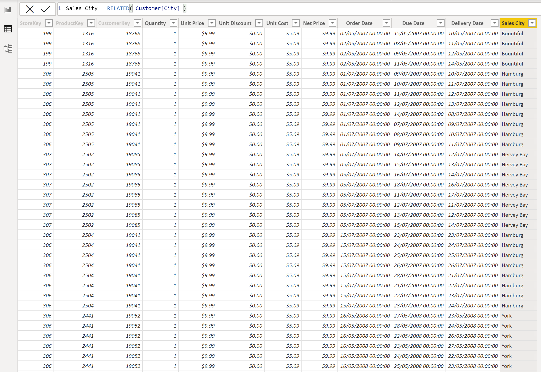
To do this, we can use the RELATED function to create a new calculated column in the 'Sales' table:

Sales City = RELATED( Customer[City] )

For each row in the 'Sales' table, RELATED will perform a look-up in the 'City' column of the 'Customer' table, and return the single related value.

If we did not use RELATED in our calculated column expression, then we would get an error. This is because, in Power BI, the row context does not propagate through relationships. When you create a formula in a calculated column, the row context for that formula includes the values from all columns in the current row of the same table. The reason RELATED allows you to perform look-ups in other tables, is because the RELATED function expands the context of the current row to include values in a related column of another table.

RELATEDTABLE

The RELATEDTABLE function works in the opposite direction to RELATED. The RELATEDTABLE function starts from the table on the one-side of the relationship and gives access to the table on the many-side of the relationship. RELATEDTABLE is a table function, and returns a table of values that contains all of the rows on the many-side that are related to the current row on the one-side.

To use the RELATEDTABLE function, you specify the table name that contains the related data that you want.

RELATEDTABLE(<tableName>)

Using RELATEDTABLE

Now let's demonstrate how we can use the RELATEDTABLE function to calculate the number of sales made by each customer.

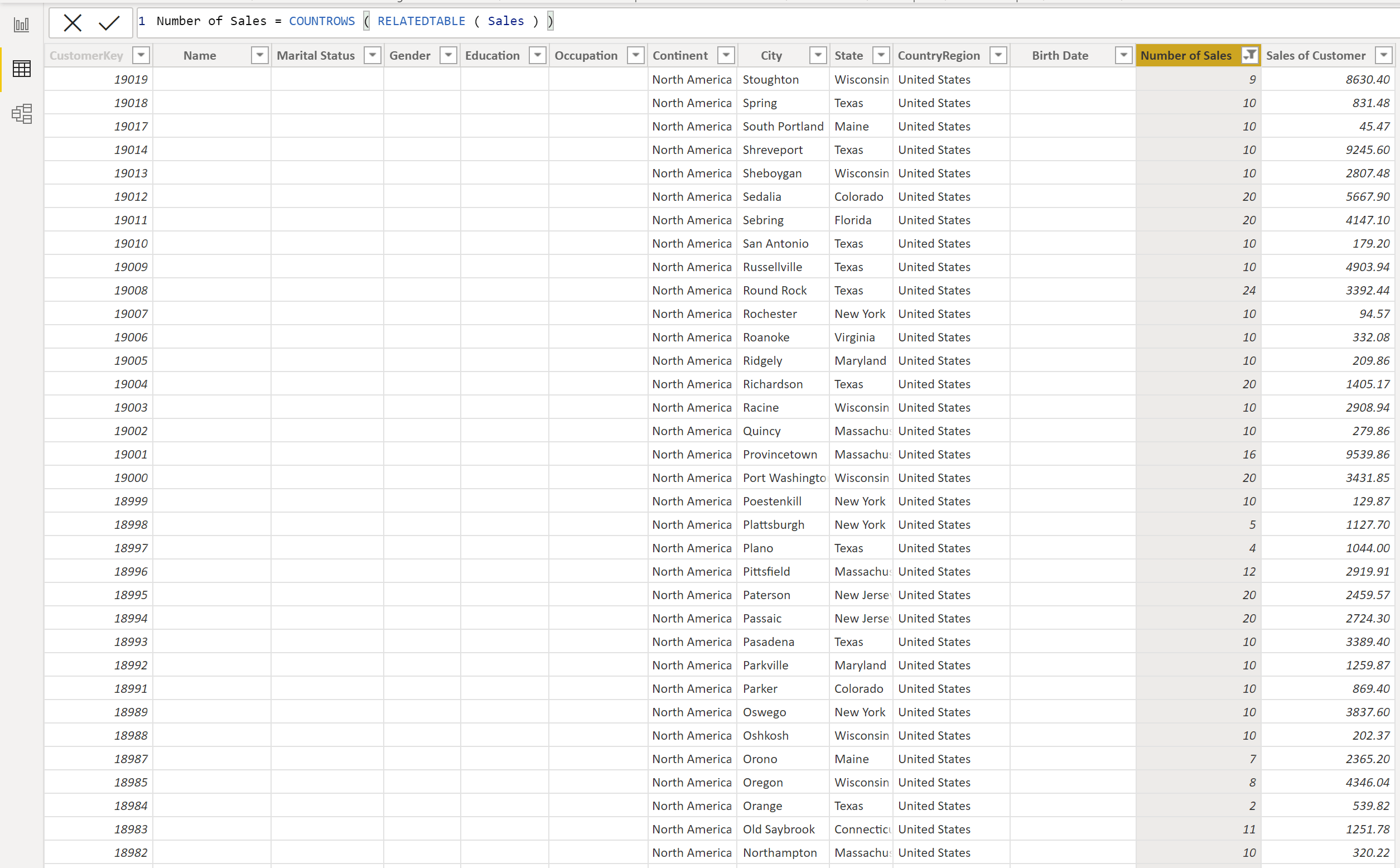
To do this, we can use the RELATEDTABLE function to create a new calculated column in the 'Customer' table:

Number of Sales = COUNTROWS ( RELATEDTABLE ( Sales ) )

Here, for each customer, RELATEDTABLE will return a sub-set of the 'Sales' table that only includes rows related to that customer. COUNTROWS will then simply count the number of rows in this sub-table. As a result, the calculated column will display number of rows in the 'Sales' table that are related to each customer.

Let's go one step further. What if now, instead of counting the sales made by each customer, we want to compute the total amount sold to each customer?

To do this, we can use the RELATEDTABLE function to create a new calculated column in the 'Customer' table and show the total sales amount for each customer:

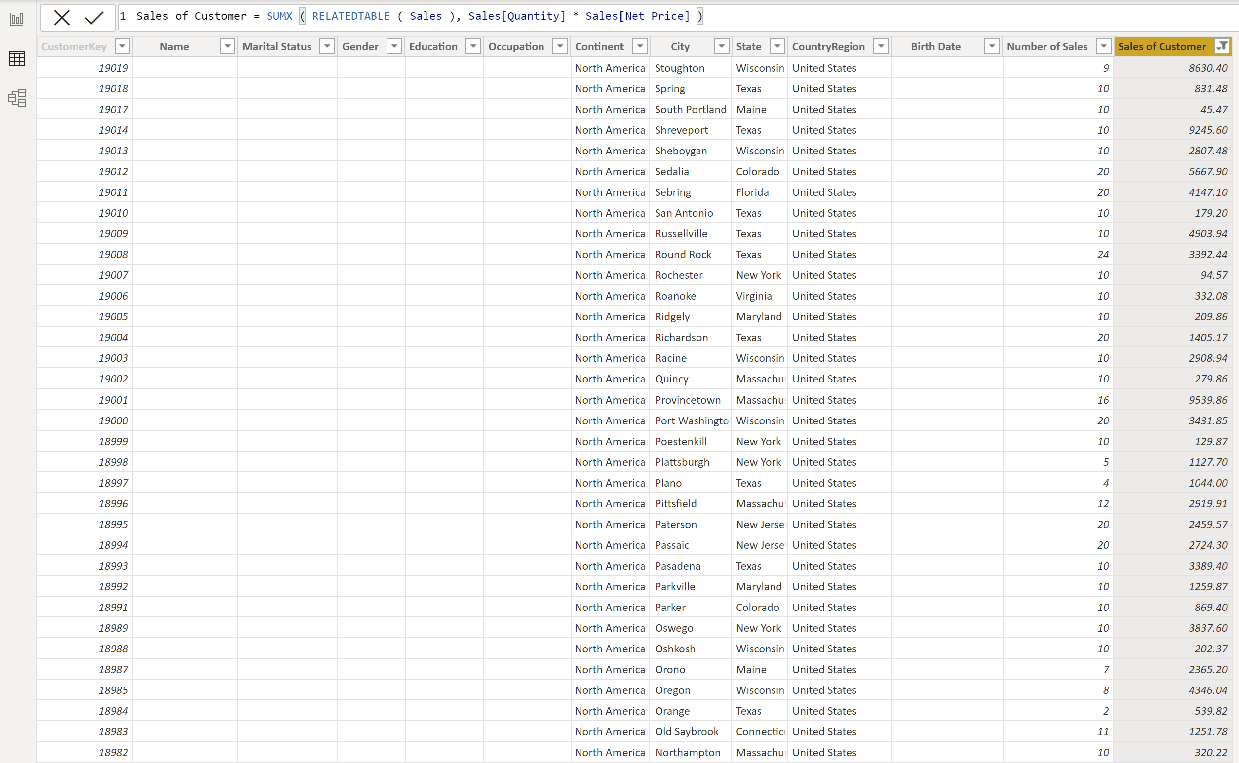
Sales of Customer = SUMX ( RELATEDTABLE ( Sales ), Sales[Quantity] * Sales[Net Price] )

In order to calculate the sales amount for each customer, we need to first find all of the transactions made by each customer. So, for each record in the 'Customer' table, RELATEDTABLE will travel through the existing relationship between the tables, and will populate a list of rows (a sub-table) from the 'Sales' table. This sub-table contains all of the sales related to that specific customer in the sales table. This table is then used as the input for the SUMX function. For each row in the sub-table, the sales amount is calculated using the SUMX iterator, and is then aggregated to give a total sales amount for that customer which is displayed in the new calculated column in the 'Customer' table.

Here, you can see the combination of: a calculated column, an expression, an iterator (SUMX) and a table function (RELATEDTABLE) together, allowing us to enrich the 'Customer' table with interesting information.

Conclusion

In this blog post, we have seen how the RELATED function can look-up values in the one-side, to populate the many-side, and we have also seen how the RELATEDTABLE function returns a table of values from the many-side, to the one-side.