Measures vs Calculated Columns in DAX and Power BI

Measures and calculated columns both use DAX expressions. You can compute values using calculated columns or using measures. This blog post will explain the difference between a calculated column and a measure and when you should use each one respectively.

What is the difference between a measure and a calculated column?

Calculated columns are computed based on data that has already been loaded into your data model. When you write a calculated column formula, it is automatically applied to the whole table and evaluated individually for each row. The values in calculated columns are evaluated when you first define them and when you refresh your dataset. Once evaluated, the values are stored in your data model, which means your data model size increases and it consumes more RAM. The more calculated columns you have the larger your model will become. On the other hand, measures are computed at query time. A measure is stored in the model as source code, but it is computed only when it is used in the report.

Another important difference between measures and calculated columns is that measures are evaluated in the filter context of the visual in which they are applied. The filter context is defined by the filters applied in the report such as row selection, column selection, report filters and slicers applied. Measures are only evaluated at the level of granularity they are plotted at. As calculated columns are computed when you first define them/ when you refresh your dataset, they do not have access to the filter context. Calculated columns are calculated outside of the filter context and do not depend on user interaction in the report.

When you write a calculated column, you need to rely only on the row context. The row context, is simply the notion of a current row. It specifies which row we are calculating the values for, so that DAX can look at other values in the same row. In a calculated column, the row context is implied. When you write an expression in a calculated column, the expression is evaluated for each row of the table. The calculated column has knowledge of the current row.

By contrast, measures implicitly do not have a row context. This is because, by default, they work at the aggregate level. So, you cannot refer to columns directly in a DAX measure, you will get an error because no row context exists. This is because the measure will not know which row to choose in the table. In order to reference a column in a measure, you must wrap the column in an aggregation function. As we are aggregating values, it doesn't matter which row we are using, we do not need a row context, as we are just aggregating all of the values in a single column to return a single value. Alternatively, we can create a row context in a measure by using an iterator function. This topic will be explained further in the following section.

Aggregation functions and iterator functions

Aggregation functions are a set of functions that aggregate the values of a column in a table and return a single value. There are many aggregation functions such as SUM, AVERAGE, MIN and MAX and their behaviour changes only in the way they aggregate values. For example, SUM adds values, whereas AVERAGE returns the average value and MIN returns the minimum value, and so forth.

The standard aggregator, SUM, aggregates all the rows of a table if it is used in a calculated column. Whenever it is used in a measure, it considers only the rows that are being filtered by slicers, rows, columns and filter conditions in the report (the filter context).

There is a strong limitation to these standard aggregation functions. They can only aggregate values from a single column. By contrast, some aggregation functions can aggregate an expression, instead of a single column. These are known as iterators.

Iterator functions are particularly useful when you need to make calculations using multiple columns or different related tables. Some common iterators include: SUMX, AVERAGEX, MINX and MAXX. Iterators accept at least two parameters. The first is a table that they scan, the second is typically an expression that is evaluated for each row of the table. This expression can be a calculation that includes multiple columns of a table. Once iterators have evaluated the expression for each row in the table, iterators then aggregate the results.

Indeed, the standard aggregation functions are simplified versions of their X-suffixed iterator counterparts. For example, the expressions specified below are two different ways of computing the same aggregation for a single column. They will return the same aggregation value.

SUM ( Sales[Quanity] )` and `SUMX ( Sales, Sales[Quantity] )

Thus, the fundamental difference between standard aggregators and their equivalent iterators is that iterators have the additional functionality of being able to aggregate expressions, rather than just a single column (Note that some iterators do not correspond to any aggregator).

Iterator functions are particularly useful when trying to avoid creating expensive calculated columns. For example if we wanted to compute the average number of days an order takes to deliver we could achieve this via the following two expressions:

We could first create a calculated column which computes the number of days to deliver an item using the following expression:

Days to Deliver = Sales[Delivery Date] - Sales[Order Date]

We would then need an additional measure which computes the average value by averaging the calculated column. The aggregation function AVERAGE shows the days to deliver for each order, and then computes the average of all the durations at the grand total level:

Average Days to Deliver = AVERAGE ( Sales [Days To Deliver] )

Alternatively, you can accomplish the same result in one measure by simply using the iterator counterpart AVERAGEX:

Average Days to Deliver =
AVERAGEX (
    Sales,
    Sales[Delivery Date] - Sales[Order Date]
)

AVERAGEX can iterate the Sales table and compute the days to deliver for each row, averaging the results at the end. By contrast, in the original example, AVERAGE cannot average an expression, so a calculated column is required to compute the expression. AVERAGEX can do this because using an iterator function introduces a row context to the measure. AVERAGEX has knowledge of the current row of the table, thus it is able to compute an expression for each row of the table.

The main advantage of using iterator functions over the standard aggregation function, is that they allow you to create measures that can aggregate expressions by introducing a row context. Thus, removing the reliance on an expensive calculated column which uses more disk space.

An example of where you could use either a measure or a calculated column to compute the same result

To illustrate a scenario where you could use either a measure or a calculated column to compute the same result I have generated a simple Power BI report that provides sales information for different products in a supermarket. Here, I have a calculated column and a measure that both compute the sales amount (£) for each different product. When I place the measure and the calculated column onto the table visual the result is identical.

Although they compute the same result, internally, they are behaving differently. So let’s explore their different behaviour by looking at the measure ‘Sales Amount’ first:

Sales Amount = SUMX ( Sales, Sales[Quantity] * Sales[Net Price] )

As measures, by default, do not have a row context, the measure uses the iterator function SUMX in order to create a row context. SUMX will iterate through each row of the visual in which the measure is applied one by one and will apply the formula in that row. It will then will aggregate all of the results at the end by adding up all of the values in each row to produce a total sales amount.

On the other hand, the expression for the calculated column ‘Line Amount’ is as follows:

Line Amount = Sales[Quantity] * Sales[Net Price]

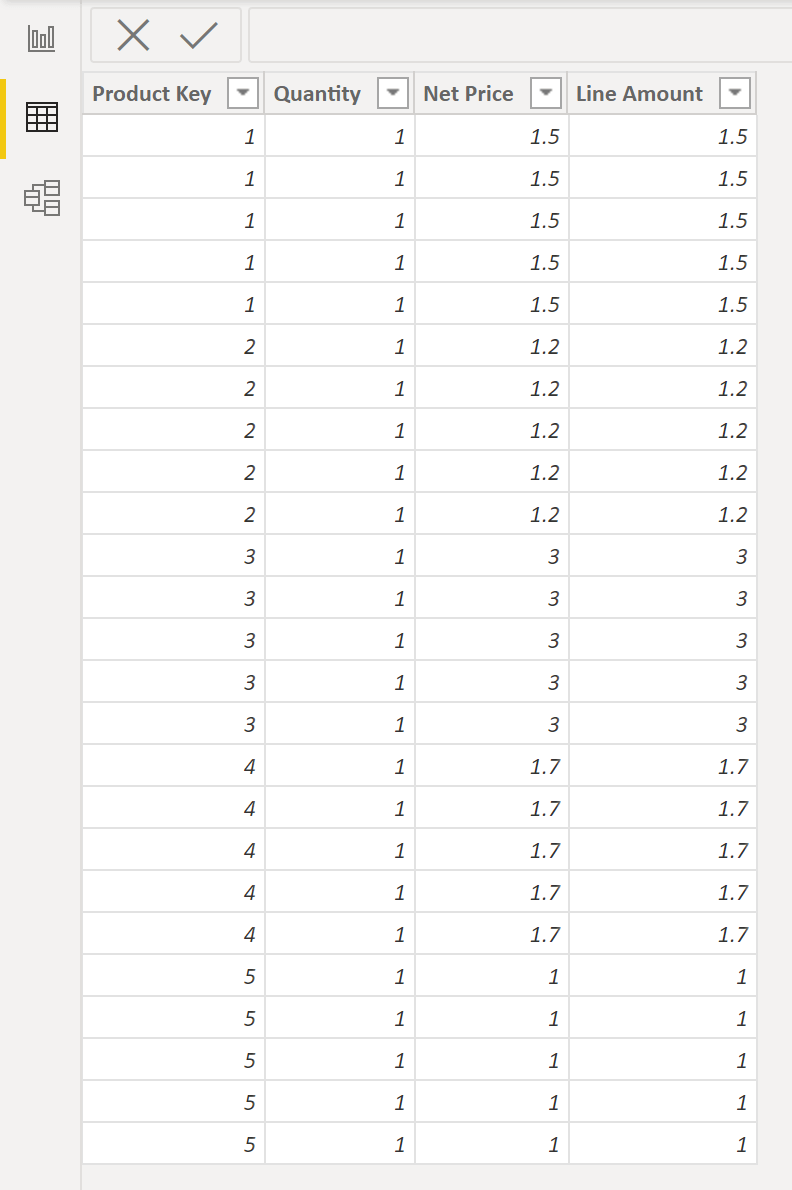
The calculated column has a row context, it has the notion of current row, so no aggregator wrapper around the expression is needed. The expression above is evaluated for each row of the table. If we look at the table view of the model we can see this in action. For each row in the Sales table, Quantity and Net Price are multiplied together to produce a Line Amount. These values are stored within the model in a new calculated column called Line Amount.

When to use a measure vs. when to use a calculated column?

When you are doing computations where using either a measure or a calculated column is an option, such as in the example above, as a general rule, you should choose measures. When it comes to doing calculations of numbers that you want to build into your report and add to visuals, then measures are typically preferred. This is because measures only use CPU, whereas calculated columns use space on both disk and RAM. Thus, it is more space and memory efficient to avoid using calculated columns. This becomes more crucial the larger the dataset.

That said, if these calculations are large and complex, you might need to pre-compute intermediate values in a calculated column. In this scenario, having the expression evaluated at data refresh using a calculated column rather than at query time using a measure may result in a better user experience. In this case, improvements to the user experience through not having to wait for the calculation at query time may outweigh the cost of using more space in your model.

In other scenarios, the kind of computation you are doing will determine whether you will use a measure or calculated column. In these scenarios you cannot choose between the two. For some calculations, you can only use a calculated column to achieve the desired result, and similarly, for other calculations, you can only use a measure. For example, if you need to operate on aggregate values instead of on a row-by-row basis you will need to use a measure. For example, when computing the aggregate value of a percentage. Calculated columns cannot be used to perform this calculation as you cannot use an aggregation of calculated columns.

Alternatively, you will need to use calculated columns if the physical structure of the calculated column is required. For example, if you need to place the calculated results in a slicer or if you need to use the result as a filter condition, you will have to create a calculated column as you cannot filter/slice by a measure. Another scenario where you can only use a calculated column is if you want to categorize text or numbers.

Conclusion

We have seen how measures and calculated columns can be used to compute values in DAX and Power BI. We have seen that calculated columns are computed when you first define them and at dataset refresh, whereas measures are computed at query time when they are applied to the report. We have also seen that measures are only evaluated at the level of granularity they are plotted at, considering only the rows that are being filtered by slicers, rows, columns and filter conditions in the report (the filter context). Whereas, calculated columns are computed outside of this filter context, and depend only on the row context, which is simply the knowledge of the current row. We have seen how measures, by default, do not have a row context and are computed at the aggregate level, therefore column references need to be wrapped in aggregation functions. We have seen how iterator functions can be used to generate a row context in a measure.

Finally, we have seen that the choice between using a measures vs. a calculated column depends on a variety of factors. When executing a calculation that could either use a measure or a calculated column, you should generally opt for measures, as calculated columns use space in your model and consume both disk space and RAM. However, in some scenarios, you cannot use a measure, and a calculated column is required, such as where you require the physical structure of the calculated column.