Providing comparative context with DAX Calculated Tables under Row Level Security


Row Level Security (RLS) in Power BI is the right way to restrict access to data in your reports based on the users' context. It is applied at query time, meaning the data isn't present in the model by the time a user accesses the tables, so there's no chance of data leakage. But this presents challenges when your users need comparative context from data they can't see - for example a global average. This post walks through a pattern using DAX to create Calculated Tables to give restricted users meaningful benchmarks without exposing the underlying data.
The comparative data problem with RLS
Let's start by describing the issue with a simple example. Consider a retail chain with twelve regional managers, each managing ten stores. They have access to a sales report to understand how their stores are performing, but RLS has been used to filter the report data so each manager can only see their own stores sales performance. With RLS in effect, there's no way for them to see how they're performing against the regional or company average. RLS solves one problem (who sees what) but introduces another (comparison becomes invisible).
We've seen this scenario show up many times and in many ways over the years. We've also seen lots of workarounds - duplicating reports for each audience, manual exports of aggregated data, or ad-hoc report requests from the BI team. None of these solve the problem properly - they add maintenance overhead, fragment the analysis and result in potentially stale data.
But, there is a cleaner pattern that solves the problem without the need for duplicating reports or business logic. We can use DAX Calculated Tables to pre-aggregate data at refresh time to a level that is inherently safe to share with all users, regardless of their RLS role. The sensitive detail never surfaces, but the comparative context becomes available to everyone.

Why common approaches fall short
Before we look at calculated tables, let's first understand why other approaches break down.
Using ALL() or ALLEXCEPT() in measures
Often people look for DAX measure-level fixes. The instinct is to write a measure using ALL() or ALLEXCEPT() to remove the RLS filter context.
However, this approach does not work - RLS filters are applied at the storage engine level, before DAX executes. By the time your measure runs, the filter is already in place. ALL() can only remove filters that DAX itself added (from visuals, slicers, or CALCULATE context). It has no access to security filters and cannot remove them.
Beware - confusion typically surfaces during development as report authors test measures in Power BI Desktop, where RLS is not enforced (unless using the View As functionality to test RLS rules), and ALL() appears to work correctly. When the same report is viewed by a restricted user with RLS, the measure returns only their filtered data - not the global values they expected.
Separate reports per audience
Another approach is to build separate reports for different audiences at different levels of aggregation - e.g. one for regional managers, another for country managers, another for executives. This works, but the cost is high, and users cannot compare reports side-by-side. Any changes or fixes to DAX logic or report visuals require updates in multiple places.
Hardcoded summary tables
Alternatively, we could load pre-aggregated data directly from the source system, hardcoded at load time. This might be in a data processing pipeline outside of Power BI, or it might be within Power Query transformations. But this is a brittle approach - the moment the underlying measure logic changes (someone fixes a measure definition or corrects historical data), the hardcoded summary becomes stale and needs re-calculating.
The recommended pattern: DAX calculated tables
A DAX Calculated Table is a table defined in the Power BI data model using DAX expressions. It is computed once, at model refresh time, and stored in the model. Visuals and measures then reference it like any other table.
The key advantage here is timing - because the calculated table is computed at refresh time, not at query time, RLS filters do not apply to it. Every user sees the same calculated table. But if we design the table to contain only aggregated data (averages, totals at a safe hierarchy level, counts), we expose nothing that should be confidential.
The pattern works like this:
- We identify the hierarchy levels in our data that are safe to share across all users (region, global etc.).
- We define a calculated table that aggregates measures to those safe levels only. The sensitive detail (individual stores, individual transactions) never appears in the table.
- We write measures that reference this table for comparison. These measures are used in visuals alongside the standard RLS-filtered data.
- The result is a report where each user sees their own data in full, plus comparative benchmarks that are appropriate for their role.
This helps to unlock comparative analysis without compromising security. The business logic lives in the existing measures, so the model stays maintainable, and the aggregation is refreshed automatically with the rest of the model.
An example: Sales by store, region, and global
Let's make this concrete using the same retail scenario.
The data model
We have a Sales fact table with:
StoreID,RegionID,SalesAmount,Date
And a Store dimension with:
StoreID,StoreName,RegionID,RegionName
The RLS role "Region Manager" applies a filter rule to the Store table: RegionID = [UserRegion], where UserRegion is a parameter passed from the application context.
We also have a Total Sales measure, defined as:
Total Sales = SUM(Sales[SalesAmount])
The calculated table
Now we define a calculated table called AggregatedBenchmarks. This table will contain regional averages and a global average, computed at refresh time:
AggregatedBenchmarks =
UNION(
    -- Regional averages
    SELECTCOLUMNS(
        VALUES(Store[RegionName]),
        "Level", "Region",
        "Label", Store[RegionName],
        "Average Sales", CALCULATE(
            AVERAGEX(VALUES(Store[StoreID]), [Total Sales]),
            ALLEXCEPT(Store, Store[RegionName])
        )
    ),
    -- Global average
    ROW(
        "Level", "Global",
        "Label", "All Regions",
        "Average Sales", CALCULATE(
            AVERAGEX(VALUES(Store[StoreID]), [Total Sales]),
            ALL(Store)
        )
    )
)
This table is computed once at model refresh time. Because RLS filters do not apply at refresh time, ALL() and ALLEXCEPT() work as expected - they can traverse the full dataset to produce correct aggregates for every region and the global total.

However, AggregatedBenchmarks is not itself protected by RLS. Without additional security, every user can query every row in the table, meaning a regional manager would see the averages for all other regions, not just their own. Whether this is acceptable depends on your requirements.
If regional averages are considered sensitive, apply an RLS filter to AggregatedBenchmarks that restricts each user to their own region's row plus the global row:
[Level] = "Global" || [Label] = LOOKUPVALUE(Store[RegionName], Store[RegionID], [UserRegion])
If regional averages are not considered sensitive (i.e. only store-level transaction detail is), then no additional RLS on the calculated table is needed, and all users can see all benchmark rows. This is often acceptable and is part of what makes the pattern useful: aggregated benchmarks can be shared safely, even when the underlying detail cannot.
The full data model looks like this:
flowchart TD
    subgraph Facts["Fact Tables"]
        Sales["**Sales**<br>StoreID<br>RegionID<br>SalesAmount<br>Date"]
    end

    subgraph Dimensions["Dimension Tables"]
        Store["**Store**<br>StoreID<br>StoreName<br>RegionID<br>RegionName"]
    end

    subgraph Calculated["Calculated Tables — computed at refresh"]
        AggBench["**AggregatedBenchmarks**<br>Level<br>Label<br>Average Sales"]
    end

    RLS1["RLS Filter — Store<br>RegionID = UserRegion"]
    RLS2["RLS Filter — AggregatedBenchmarks<br>Level = 'Global'<br>OR Label = UserRegionName"]

    Sales -->|"many-to-one (StoreID)"| Store
    RLS1 -->|"filters at query time"| Store
    Store -.->|"aggregated at refresh<br>(RLS does not apply)"| AggBench
    RLS2 -->|"filters at query time"| AggBench
The comparison measures
We can now write two simple measures that read directly from AggregatedBenchmarks:
Regional Average Sales =
CALCULATE(
    MAX(AggregatedBenchmarks[Average Sales]),
    AggregatedBenchmarks[Level] = "Region"
)

Global Average Sales =
CALCULATE(
    MAX(AggregatedBenchmarks[Average Sales]),
    AggregatedBenchmarks[Level] = "Global"
)
Both measures read from the pre-computed table rather than recalculating from the underlying data - this is the critical distinction.
N.B. For Regional Average Sales, the measure depends on the RLS filter on AggregatedBenchmarks being in place. With that filter applied, each user sees only their own region's row at Level = "Region", so MAX returns the correct single value. Without it, the measure would return the highest regional average across all regions rather than the current user's. If you chose not to apply RLS to AggregatedBenchmarks, this measure would need to be rewritten to identify the user's region explicitly (for example, using LOOKUPVALUE to match on the user's region). For Global Average Sales, the Level = "Global" filter targets the single pre-computed global row, which is always visible regardless of the user's RLS role.
The final report
A complete working example of this pattern is available to download from GitHub.
endjin/pbi-rls-calculated-tables
The report is in the Power BI project format (.pbip) and can be opened directly in Power BI Desktop (November 2023 or later). It uses hardcoded sample data - nine stores across three regions (North, South, and East), so no data source connection is required.
Three RLS roles are defined, one per region:
- North Region Manager — restricts to Store A, Store B, and Store C
- South Region Manager — restricts to Store D, Store E, and Store F
- East Region Manager — restricts to Store G, Store H, and Store I
Each role also applies the corresponding filter to AggregatedBenchmarks, so users see only their own regional average alongside the global average.
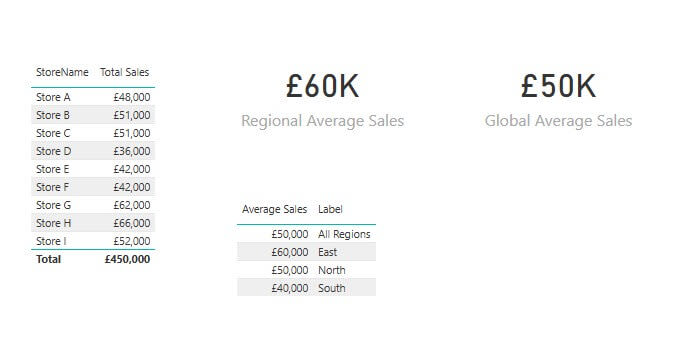
To explore the report, open it in Power BI Desktop and use Modelling → View as to switch between roles. Without any role applied, all nine stores are visible and all three regional averages appear in the benchmark table - this represents the admin or unrestricted view.
Switching to the South Region Manager role restricts the store table to the three South stores. The Regional Average Sales card updates to reflect the South average (£40,000), while the Global Average card remains unchanged (£50,000). The benchmark table shows only the South row and the global row - the North and East regional averages are filtered out.
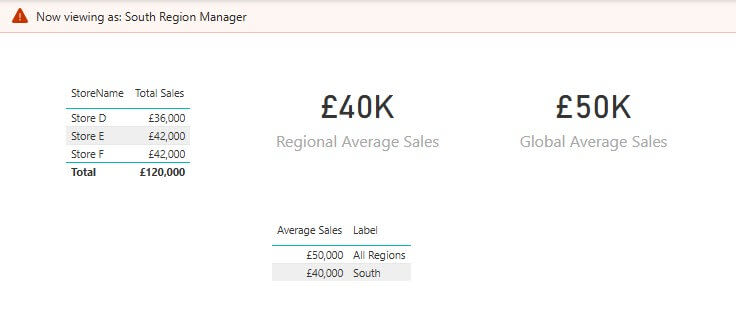
The North and East roles behave identically, scoped to their respective stores and regional averages.
The store table and benchmark cards are driven by entirely separate parts of the model - the former by RLS-filtered data from Sales and Store, the latter by the pre-computed AggregatedBenchmarks table. This separation is what makes the pattern work.
When to apply this pattern
This pattern works well when:
- Your hierarchy has clear safe levels. There is a well-defined aggregation level (region, country, global) where data can be shared across users without exposing sensitive detail.
- Your measures are stable and worth reusing. Business logic lives in one place. If the
Total Salesdefinition changes, the calculated table automatically reflects the updated logic at next refresh. - Different users have genuinely different data rights. The pattern is most valuable when RLS creates a real visibility gap - users who need comparative context but cannot see the underlying detail.
- Real-time comparison is not a requirement. Benchmarks are computed at model refresh. Daily or weekly refresh cycles are typically sufficient for this kind of analysis.
- Your hierarchy is likely to grow. Adding a new level (business unit, product category) requires only a small addition to the
UNION()call. The pattern extends naturally without restructuring the model. - You need benchmarks for multiple metrics. Additional aggregated measures are added by including new columns in the
ADDCOLUMNS()calls. All benchmarks live in a single table, keeping the model coherent and the benchmark logic easy to find.
This pattern is less suitable when:
- Your hierarchy is highly dynamic. If new levels or branches are added frequently, maintaining the calculated table definition becomes overhead.
- Your data model is already very large. Every aggregated row is stored in the model. In high-cardinality, multi-dimensional hierarchies, the calculated table can grow quickly.
- The aggregation logic diverges from your measures. If the benchmarks require substantially different calculation logic from your existing measures, the reuse benefit is lost and the pattern adds complexity without a clear return.
Summary
Row Level Security in Power BI is essential for controlling who sees what. But security constraints often come at the cost of comparative insight. Users locked into their own data cannot easily benchmark themselves against the wider dataset.
DAX Calculated Tables offer a clean solution. By pre-aggregating data to safe hierarchy levels at refresh time, we expose only what we intend to share, and we reuse existing business logic to do it. The pattern is straightforward to implement, maintainable, and scales well to typical organisational structures.